Dashing Through Search Spaces
in the Physical Sciences
PHD DEFENCE
University of Oslo — 7 October 2022
Jeriek Van den Abeele
16 orders of magnitude separate the Planck scale and the weak scale!
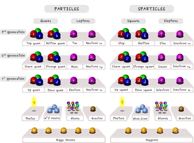
The Standard Model is incomplete.
- Extreme sensitivity to UV contributions indicates a real problem, manifest in radiative corrections to the Higgs mass
- One solution, supersymmetry, connects fermions and bosons — and introduces new particles and opportunities to explain more
- Upgrading supersymmetry to a local symmetry leads to gravitinos (supergravity)
[CERN/C. David]
Global fits address the need for a consistent comparison of BSM theories to all relevant experimental data
Challenge:
Scanning increasingly high-dimensional parameter spaces with varying phenomenology
Exploration of a combined likelihood function:
\(\mathcal{L} = \mathcal{L}_\mathsf{collider} \times \mathcal{L}_\mathsf{Higgs} \times \mathcal{L}_\mathsf{DM} \times \mathcal{L}_\mathsf{EWPO} \times \mathcal{L}_\mathsf{flavour} \times \ldots\)
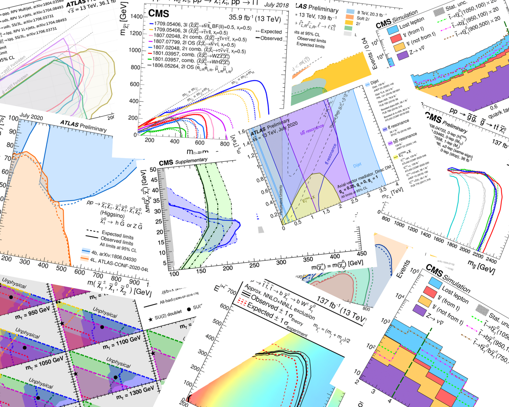
Supersymmetry turns out hard to find ...
High-dimensional search spaces are non-intuitive
Most of the volume lies in the extremities!
Adaptive sampling techniques are essential for search space exploration: differential evolution, nested sampling, genetic algorithms, ...
In a 7-dimensional parameter space, you have only covered 47.8% of the space.
In a 19-dimensional parameter space, only 13.5%. And a grid with just 2 points per dimension takes 524,288 evaluations.
Imagine scanning the central 90% of each parameter range really well, at great cost.
90%
Quick cross-section prediction with Gaussian processes
based on work with A. Buckley, A. Kvellestad, A. Raklev, P. Scott, J. V. Sparre, and I. A. Vazquez-Holm
Global fits need quick, but sufficiently accurate theory predictions
BSM scans today easily require \(\sim 10^7\) samples or more.
Higher-order BSM production cross-sections and theoretical uncertainties make a significant difference!

[GAMBIT, 1705.07919]
CMSSM

[hep-ph/9610490]

Existing higher-order evaluation tools are insufficient for large MSSM scans
- Prospino/MadGraph: full calculation, minutes/hours per point
- N(N)LL-fast: fast grid interpolation, but only degenerate squark masses
$$ pp\to\tilde g \tilde g,\ \tilde g \tilde q_i,\ \tilde q_i \tilde q_j, $$
$$\tilde q_i \tilde q_j^{*},\ \tilde b_i \tilde b_i^{*},\ \tilde t_i \tilde t_i^{*}$$
at \(\mathsf{\sqrt{s}=13} \) TeV
xsec 1.0 performs Gaussian process regression for all strong SUSY cross-sections in the MSSM-24 for the LHC

- New Python tool for NLO cross-section predictions within seconds
A. Buckley, A. Kvellestad, A. Raklev, P. Scott, J. V. Sparre, JVDA, I. A. Vazquez-Holm
- Pointwise estimates of PDF, \(\alpha_s\) and scale uncertainties, in addition to the subdominant regression uncertainty
- Future expansions: other processes, more CoM energies, higher-order corrections, ...
- Trained with Prospino results
prior distribution over all functions
with the estimated smoothness
f(\vec x) \sim \mathcal{GP}\left[m(\vec x), k(\vec x, \vec x')\right]
\mathrm{E}\left[f(\vec x)\right] = m(\vec x)
\mathrm{Cov}\left[f(\vec x), f(\vec x')\right] = k(\vec x, \vec x')
The Bayesian Way: quantifying beliefs with probability

k(\vec x, \vec x') = \sigma_f^2 \exp\left(-\frac{|\vec x-\vec x'|^2}{l^2}\right)
prior distribution over all functions
with the estimated smoothness
f(\vec x) \sim \mathcal{GP}\left[m(\vec x), k(\vec x, \vec x')\right]
\mathrm{E}\left[f(\vec x)\right] = m(\vec x)
\mathrm{Cov}\left[f(\vec x), f(\vec x')\right] = k(\vec x, \vec x')
posterior distribution over functions
with updated \(m(\vec x)\)
data
k(\vec x, \vec x') = \sigma_f^2 \exp\left(-\frac{|\vec x-\vec x'|^2}{l^2}\right)
The Bayesian Way: quantifying beliefs with probability
After optimising correlation length scales, we obtain a posterior by conditioning on known data.

target function

target function
After optimising correlation length scales, we obtain a posterior by conditioning on known data.

After optimising correlation length scales, we obtain a posterior by conditioning on known data.

After optimising correlation length scales, we obtain a posterior by conditioning on known data.
Make posterior predictions at new points by computing correlations to known points.


Make posterior predictions at new points by computing correlations to known points.
Posterior predictive distributions are Gaussian too!


[Liu+, 1806.00720]
Distributed Gaussian Processes
For standard GP regression, training scales as \(\mathcal{O}(n^3)\), prediction as \(\mathcal{O}(n^2)\).
Divide-and-conquer approach for dealing with large datasets:
- Make local predictions with smaller data subsets
- Compute a weighted average of these predictions
The exact weighting procedure is important, to ensure
- Smooth final predictions
- Valid regression uncertainties
"Generalized Robust Bayesian Committee Machine"
GP regularisation
- Add a white-noise component to the kernel
- Can compute minimal value that reduces condition number sufficiently
- Can model discrepancy between GP model and latent function, e.g., regarding assumptions of stationarity and differentiability
[Mohammadi+, 1602.00853]
- Avoid a large S/N ratio by adding a likelihood penalty term guiding the hyperparameter optimisation
- Nearly noiseless data is problematic. Artificially increasing the noise level may be necessary, degrading the model a bit
Numerical errors may arise in the inversion of the covariance matrix, leading to negative predictive variances.
Gluino-gluino production example

Gluino-squark


Squark-squark

Fast estimate of SUSY (strong) production cross- sections at NLO, and uncertainties from
- regression itself
- renormalisation scale
- PDF variation
- \(\alpha_s\) variation
Goal
$$ pp\to\tilde g \tilde g,\ \tilde g \tilde q_i,\ \tilde q_i \tilde q_j, $$
$$\tilde q_i \tilde q_j^{*},\ \tilde b_i \tilde b_i^{*},\ \tilde t_i \tilde t_i^{*}$$
Interface
Method
Pre-trained, distributed Gaussian processes
Python tool with command-line interface
Processes
at \(\mathsf{\sqrt{s}=13}\) TeV

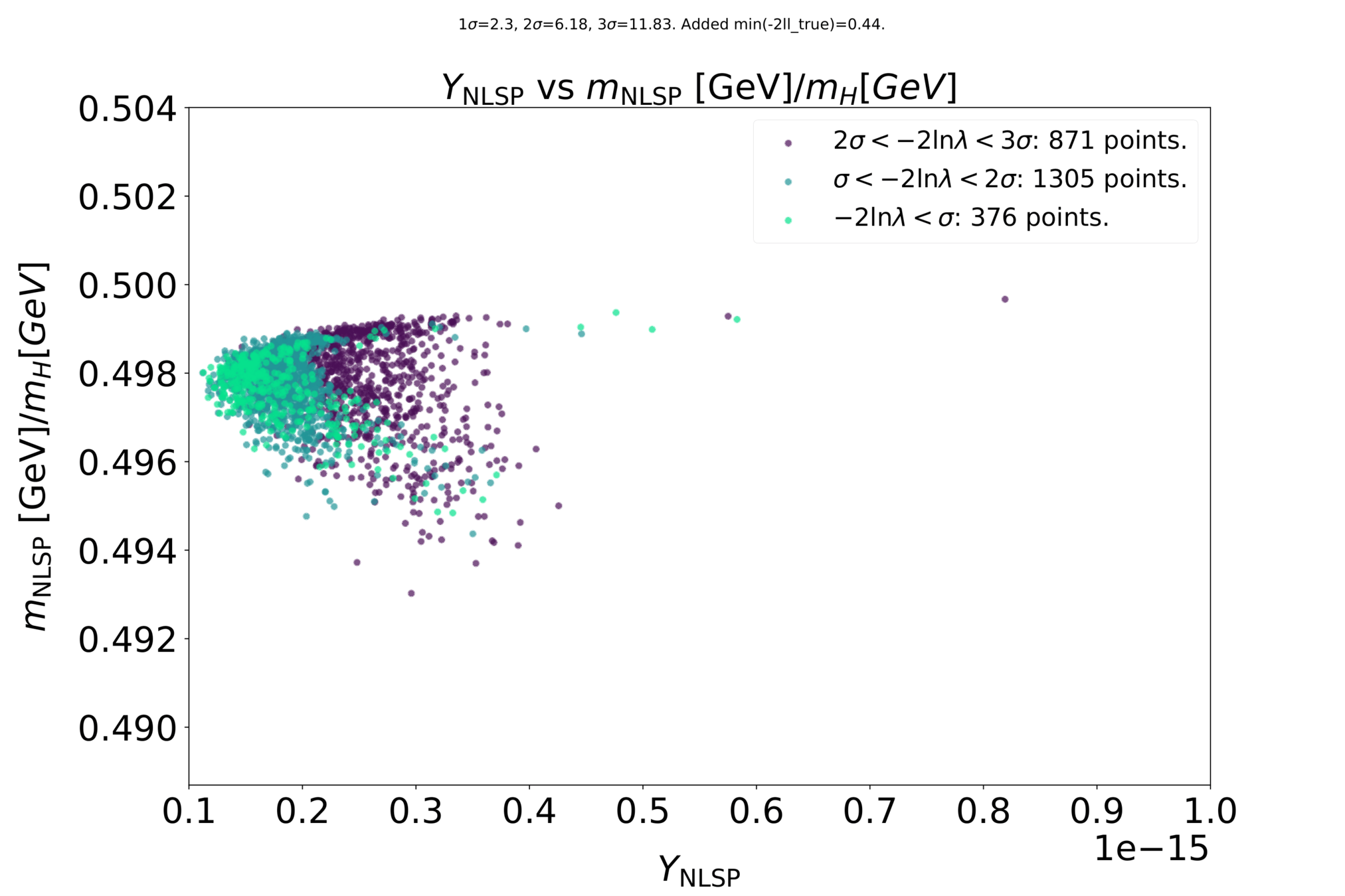
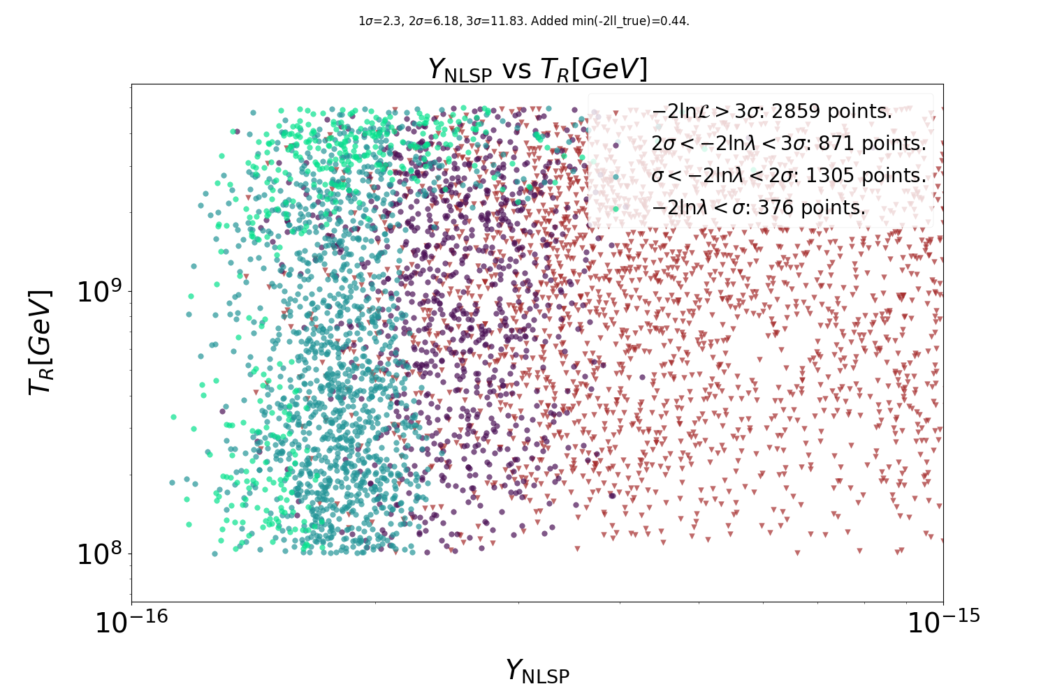
Scanning for gravitinos:
Gravitino dark matter despite high reheating temperatures
based on work with J. Heisig, J. Kersten and I. Strümke
- Planck-suppressed widths make the NLSP long-lived and a danger to BBN
- Thermal leptogenesis needs \(T_R \gtrsim 10^9\) GeV to match baryon asymmetry
-
Now, for an MSSM NLSP, thermal freeze-out (not \(T_R\)!) determines the abundance
-
\(\Omega^\mathsf{th}_\mathsf{NLSP}\) is controlled by MSSM parameters; if it is low, the BBN impact is minimal!

Given R-parity, the LSP is stable and a dark matter candidate.
In a gravitino LSP scenario:
Gravitino trouble
The heavy Higgs funnel
Parameter region where a neutralino NLSP dominantly annihilates via resonant heavy Higgs bosons: \[2m_{\tilde \chi_{1}^{0}} \approx m_{H^0/A^0}\]
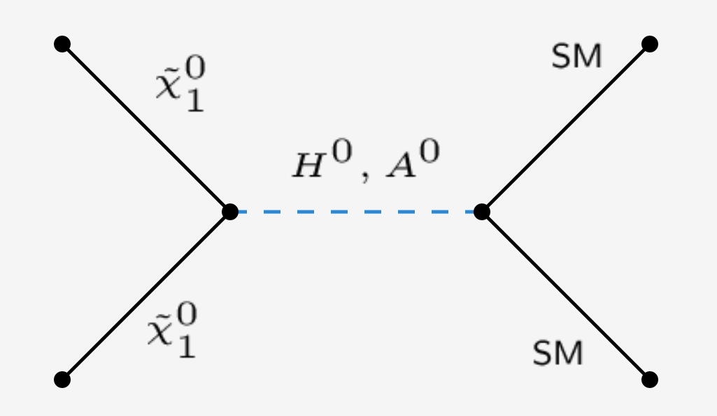
- Requires wino-higgsino NLSP
-
Open window facilitating tiny NLSP freeze-out abundance
- Avoids injecting too much energy into BBN
- Minimises non-thermal gravitino abundance contribution from NLSP decays
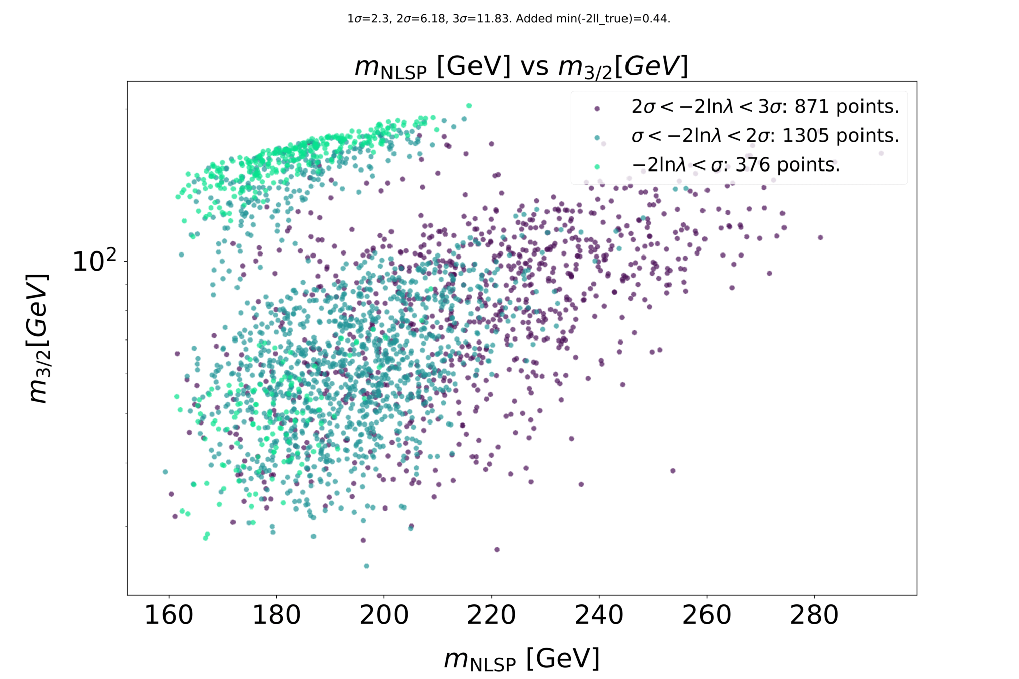
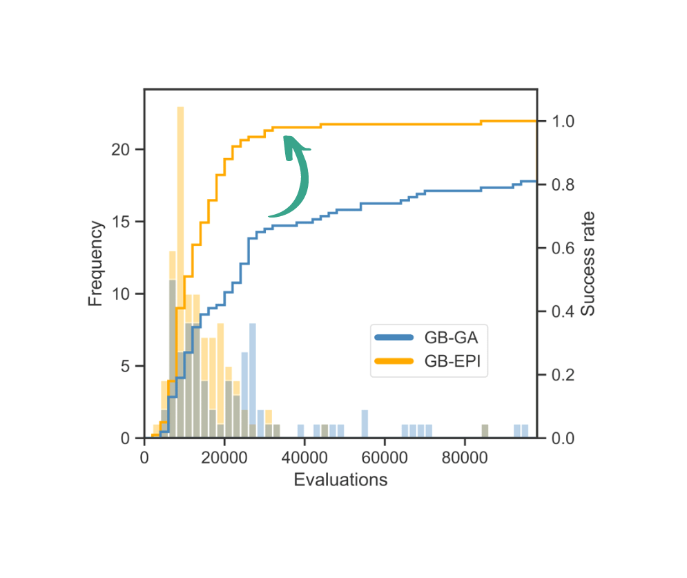
Guided scan strategy
Construct a likelihood \(\mathcal{L}_\mathsf{scan} = \mathcal{L}_\mathsf{relic\ density} \times \mathcal{L}_\mathsf{BBN} \times \mathcal{L}_\mathsf{collider} \times \mathcal{L}^\mathsf{fake}_\mathsf{T_R}\).
Nested sampling with MultiNest to examine region with highest \(\mathcal{L}_\mathsf{scan}\):
- Focusing on funnel region and guided towards high \(\mathsf{T_R}\)
- 7 parameters varied in the scan: \(T_R, m_{\tilde G}, M_1, M_2, M_3, \mu, A_0\)
- Fixed \(\tan \beta = 10\) and \(m_{scalars} = 15\ \mathsf{TeV}\)
-
External dependencies:
- SOFTSUSY (spectrum generation)
- MicrOMEGAs (thermal NLSP abundance, chargino production cross sections)
- SmodelS, CheckMATE [ROOT, Delphes, MadGraph, Pythia, HepMC] (collider checks)
Preliminary results
Scanning for gravitinos:
Light gravitinos hiding at colliders
based on work with the GAMBIT Collaboration
SUSY with a light gravitino: LHC impact
EWMSSM: MSSM with only electroweakinos (\(\tilde{\chi}_i^0, \tilde{\chi}_i^\pm\)) not decoupled
GEWMSSM: EWMSSM + nearly massless gravitino LSP
- The lightest EWino can decay, changing the collider phenomenology
- 4D parameter space: \(M_1, M_2, \mu\) and \(\tan\beta\)
- Gravitino mass fixed to 1 eV, so the lightest EWino decays promptly
- Scan with ColliderBit, using differential evolution (Diver)


Profile likelihood ratio shows preference for higgsinos near 200 GeV
(tiny excesses in searches for MET+leptons/jets)
Preliminary results
Preliminary results
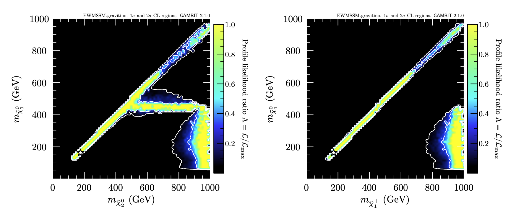
Profile likelihood ratio, with likelihood capped at SM expectation (no signal)
- Besides higgsinos, also light/lonely bino NLSP (low production cross-section)
- Large part of parameter space excluded (mostly due to photon+MET searches)
Illuminating molecular optimisation
based on work with J. Verhellen

Developing new drugs is an expensive process, typically taking 10 - 15 years.
Simple rules of thumb only provide little guidance in small-molecule drug design.
AI techniques, leveraging increased computational power and data availability, promise to speed it up.
Graph-based Elite Patch Illumination (GB-EPI) is a new illumination algorithm, based on MAP-ELITES from soft robot design.

Traditional graph-based genetic algorithm
Frequent stagnation!
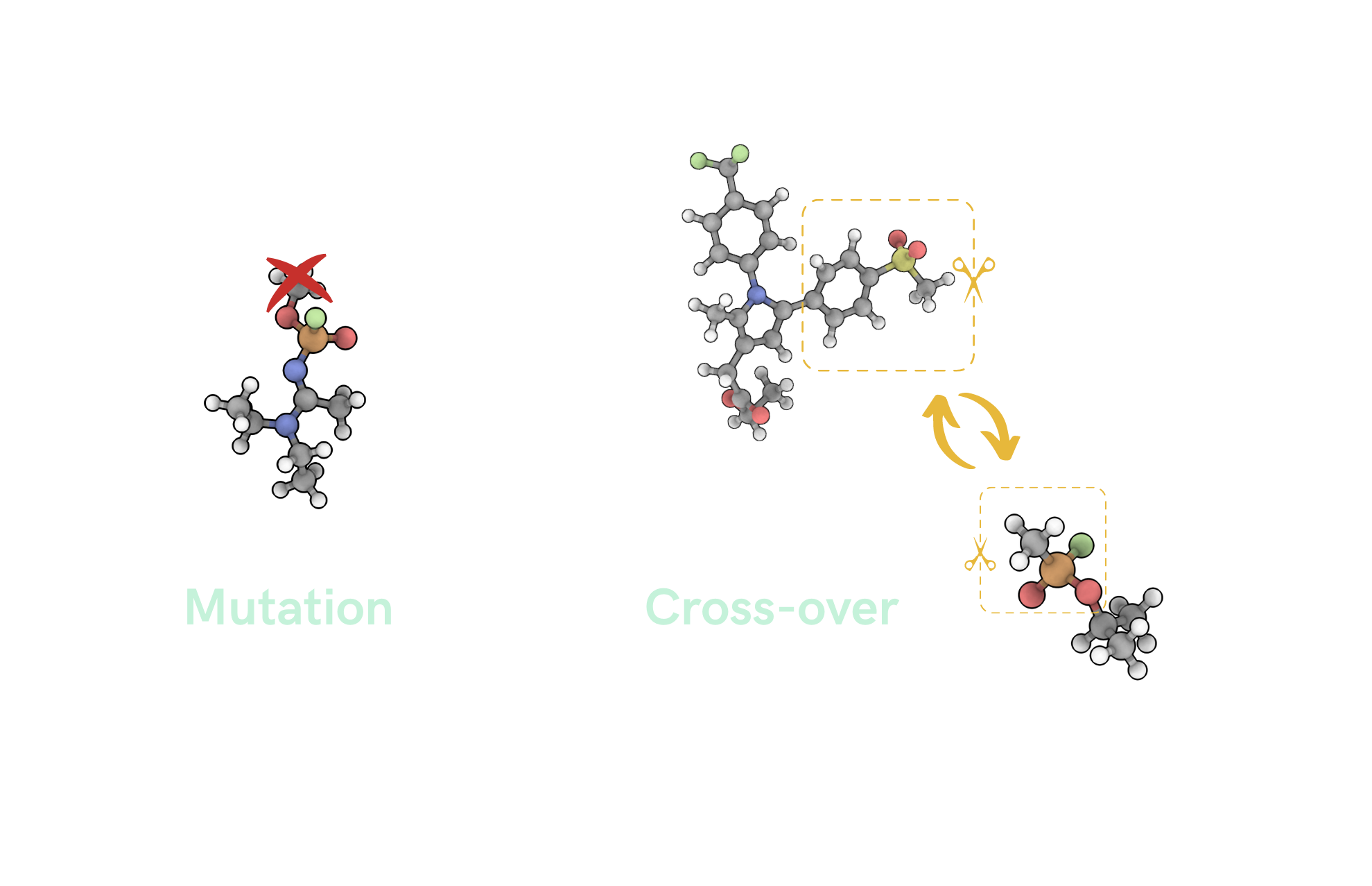

Graph-based Elite Patch Illumination
Explicitly enforcing diversity in chosen feature space!
GB-EPI illuminates search spaces: it reveals how interesting features affect performance, and finds optima in each region
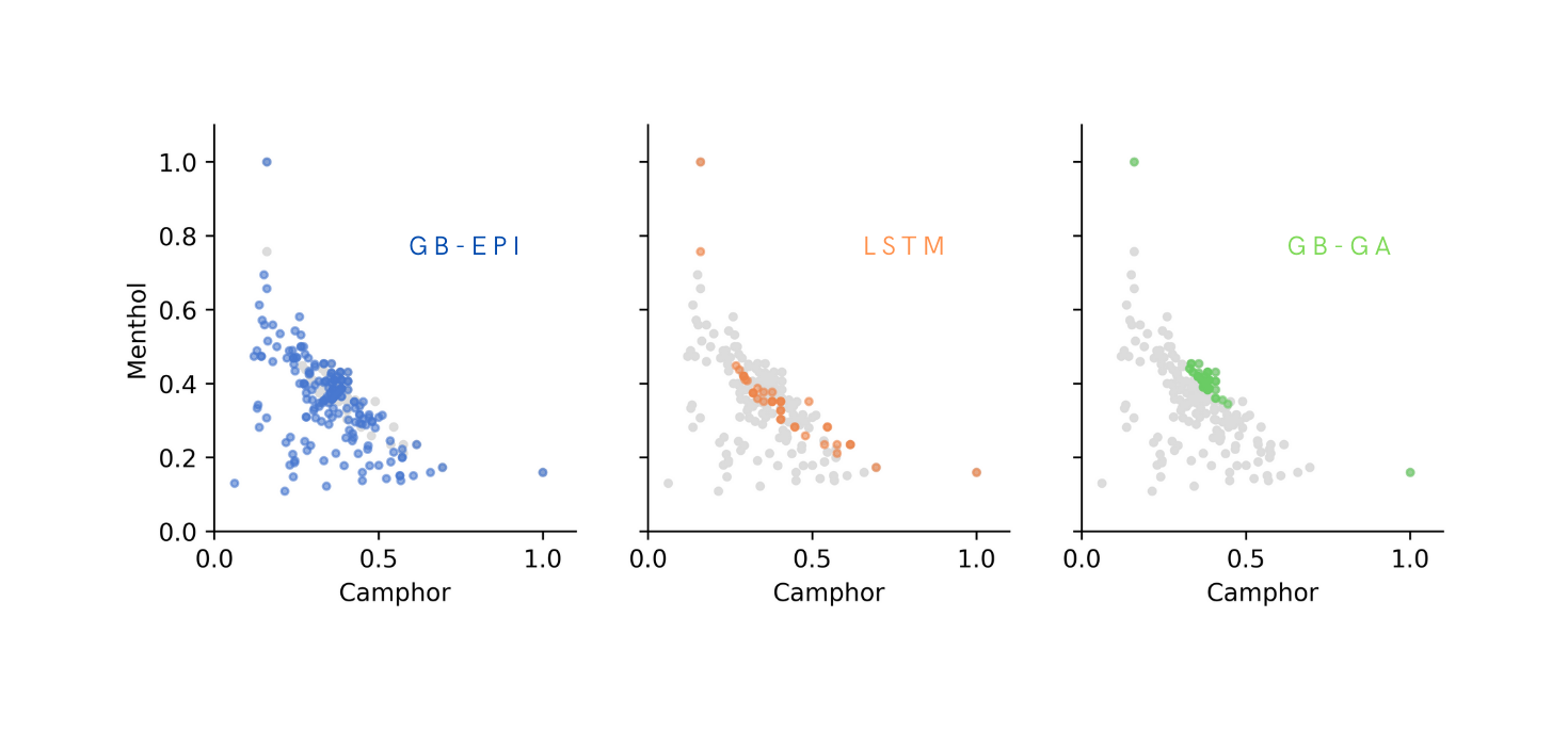
Benchmarks show that the quality-diversity approach boosts speed and success rate
- Supersymmetry is not dead.
- With increasing data and processing power, AI techniques can accelerate search space exploration.
- Looking beyond field boundaries can be fun!
Closing remarks
Thank you!


Backup slides
Let's make some draws from this prior distribution.

Let's make some draws from this prior distribution.

Let's make some draws from this prior distribution.

Let's make some draws from this prior distribution.

Let's make some draws from this prior distribution.

At each input point, we obtain a distribution of possible function values (prior to looking at data).


At each input point, we obtain a distribution of possible function values (prior to looking at data).

A Gaussian process sets up an infinite number of correlated Gaussians, one at each parameter point.
A Gaussian process sets up an infinite number of correlated Gaussians, one at each parameter point.

Sometimes, a curious problem arises: negative predictive variances!
It is due to numerical errors when computing the inverse of the covariance matrix \(K\). When \(K\) contains many training points, there is a good chance that some of them are similar:
\vec x_1 \sim \vec x_2 \quad \implies \quad
k(\vec x_1, \vec X) \simeq
k(\vec x_2, \vec X)
GP regularisation
Nearly equal columns make \(K\) ill-conditioned. One or more eigenvalues \(\lambda_i\) are close to zero and \(K\) can no longer be inverted reliably. The number of significant digits lost is roughly the \(\log_{10}\) of the condition number
\kappa = \frac{\lambda_\mathsf{max}}{\lambda_\mathsf{min}}
This becomes problematic when \(\kappa \gtrsim 10^8 \). In the worst-case scenario,
\kappa = N \left(\frac{\sigma_f}{\sigma_n}\right)^2 + 1
signal-to-noise ratio
number of points
GP regularisation
Squark-antisquark

Squared Exponential kernel
Matérn-3/2 kernel


Different kernels lead to different function spaces to marginalise over.
My kingdom for a good kernel ...
GPs allow us to use probabilistic inference to learn a function from data, in an interpretable, analytical, yet non-parametric Bayesian framework.
A GP model is fully specified once the mean function, the kernel and its hyperparameters are chosen.
The probabilistic interpretation only holds under the assumption that the chosen kernel accurately describes the true correlation structure.
The choice of kernel allows for great flexibility. But once chosen, it fixes the type of functions likely under the GP prior and determines the kind of structure captured by the model, e.g., periodicity and differentiability.

My kingdom for a good kernel ...

The choice of kernel allows for great flexibility. But once chosen, it fixes the type of functions likely under the GP prior and determines the kind of structure captured by the model, e.g., periodicity and differentiability.
My kingdom for a good kernel ...

The choice of kernel allows for great flexibility. But once chosen, it fixes the type of functions likely under the GP prior and determines the kind of structure captured by the model, e.g., periodicity and differentiability.
My kingdom for a good kernel ...
For our multi-dimensional case of cross-section regression, we get good results by multiplying Matérn (\(\nu = 3/2\)) kernels over the different mass dimensions:
\displaystyle k_s(\vec x, \vec x') = \prod_{d=1}^D \sigma_{f_d}^2
\left( 1 + \sqrt{3} \frac{|x'_d - x_d|}{l_d} \right)
\exp\left(-\sqrt{3}\frac{|x'_d - x_d|}{l_d}\right)
The different lengthscale parameters \(l_d\) lead to automatic relevance determination for each feature: short-range correlations for important features over which the target function varies strongly.
This is an anisotropic, stationary kernel. It allows for functions that are less smooth than with the standard squared-exponential kernel.

My kingdom for a good kernel ...
... with good hyperparameters


Short lengthscale, small noise
Long lengthscale, large noise
Underfitting, almost linear
Overfitting of fluctuations,
can lead to large uncertainties!
Typically, kernel hyperparameters are estimated by maximising the (log) marginal likelihood \(p( \vec y\ |\ \vec X, \vec \theta) \), aka the empirical Bayes method.
Alternative: MCMC integration over a range of \(\vec \theta\).
Gradient-based optimisation can get stuck in local optima and plateaus. Multiple initialisations can help, or global optimisation methods like differential evolution.
Global optimum: somewhere in between

... with good hyperparameters
Typically, kernel hyperparameters are estimated by maximising the (log) marginal likelihood \(p( \vec y\ |\ \vec X, \vec \theta) \), aka the empirical Bayes method.
Alternative: MCMC integration over a range of \(\vec \theta\).
Gradient-based optimisation can get stuck in local optima and plateaus. Multiple initialisations can help, or global optimisation methods like differential evolution.
The standard approach systematically underestimates prediction errors.
After accounting for the additional uncertainty from learning the hyper-parameters, the prediction error increases when far from training points.
[Wågberg+, 1606.03865]

... with good hyperparameters
Other tricks to improve the numerical stability of training:
- Normalising features and target values
- Factoring out known behaviour from the target values
- Training on log-transformed targets, for extreme values and/or a large range, or to ensure positive predictions
... with good hyperparameters
Workflow
Generating data
Random sampling
SUSY spectrum
Cross-sections
Optimise kernel hyperparameters
Training GPs
GP predictions
Input parameters
Linear algebra
Cross-section
estimates
Compute covariances between training points
Workflow
Generating data
Random sampling
SUSY spectrum
Cross-sections
Optimise kernel hyperparameters
Training GPs
GP predictions
Input parameters
Linear algebra
Cross-section
estimates
XSEC
Compute covariances between training points
Training scales as \(\mathcal{O}(n^3)\), prediction as \(\mathcal{O}(n^2)\)

A balancing act
Random sampling with different priors, directly in mass space
Evaluation speed
Sample coverage
Need to cover a large parameter space
Distributed Gaussian processes
Getting started with XSEC
pip install xsec
xsec-download-gprocs --process_type gg
# Set directory and cache choices
xsec.init(data_dir="gprocs")
# Set center-of-mass energy (in GeV)
xsec.set_energy(13000)
# Load GP models for the specified process(es)
processes = [(1000021, 1000021)]
xsec.load_processes(processes)# Enter dictionary with parameter values
xsec.set_parameters(
{
"m1000021": 1000,
"m1000001": 500,
"m1000002": 500,
"m1000003": 500,
"m1000004": 500,
"m1000005": 500,
"m1000006": 500,
"m2000001": 500,
"m2000002": 500,
"m2000003": 500,
"m2000004": 500,
"m2000005": 500,
"m2000006": 500,
"sbotmix11": 0,
"stopmix11": 0,
"mean": 500,
}
)
# Evaluate the cross-section with the given input parameters
xsec.eval_xsection()
# Finalise the evaluation procedure
xsec.finalise()Some linear algebra
Regression problem, with 'measurement' noise:
\(y=f(\vec x) + \varepsilon, \ \varepsilon\sim \mathcal{N}(0,\sigma_n^2) \quad \rightarrow \quad \) infer \(f\), given data \(\mathcal{D} = \{\vec X, \vec y\}\)
Assume covariance structure expressed by a kernel function, like
k(\vec x_i, \vec x_j) = \sigma_f^2\, \exp\!\left(-\frac{|\vec x_i - \vec x_j|^2}{2\mathcal{l}^2}\right) + \sigma_n^2\, \delta_{ij}
Consider the data as a sample from a multivariate Gaussian distribution
\([\vec x_1, \vec x_2, \ldots]\)
\([y_1, y_2, \ldots]\)
signal kernel
white-noise kernel
Some linear algebra
Regression problem, with 'measurement' noise:
\(y=f(\vec x) + \varepsilon, \ \varepsilon\sim \mathcal{N}(0,\sigma_n^2) \quad \rightarrow \quad \) infer \(f\), given data \(\mathcal{D} = \{\vec X, \vec y\}\)
Training: optimise kernel hyperparameters by maximising the marginal likelihood
p\left( \vec y\ |\ \vec X, \vec \theta \right)
= \mathcal{N} \left( \vec y \ |\ m(\vec X), K_{\vec\theta} \right)
y_*\, |\, \mathcal D, \vec x_* \sim \mathcal{N}\left(\mu_*, \sigma_*^2\right)
\propto |K_{\vec\theta}|^{-\frac{1}{2}}
\times \exp \left\{ -\frac{1}{2} \left( \vec y - m(\vec X) \right)^T K_{\vec\theta}^{-1}
\left(\vec y - m(\vec X) \right) \right\}
%
%%k(\vec X, \vec X)^{-1} \left( \vec y - \mu(\vec X) \right),
% k(\vec x_*, \vec x_*) - k(\vec x_*, \vec X) k(\vec X, \vec X)^{-1} k(\vec X, \vec x_*)
Posterior predictive distribution at a new point \(\vec x_*\) :
with
\mu_* = m(\vec x_*) + K_* K^{-1}(\vec{y}-m(\vec X))
%%\tilde\mu(\vec x_*) = \mu(\vec x_*) + k(\vec x_*, \vec X) k(\vec X, \vec X)^{-1}\vec{y}\\
%\tilde\sigma^2(\vec x_*) = k(\vec x_*, \vec x_*) - k(\vec x_*, \vec X) k(\vec X, \vec X)^{-1} k(\vec X, \vec x_*)
Implicit integration over points not in \(\vec X\)
\sigma_*^2 = K_{**}-K_*K^{-1}K_*^T
%%\tilde\mu(\vec x_*) = \mu(\vec x_*) + k(\vec x_*, \vec X) k(\vec X, \vec X)^{-1}\vec{y}\\
%\tilde\sigma^2(\vec x_*) = k(\vec x_*, \vec x_*) - k(\vec x_*, \vec X) k(\vec X, \vec X)^{-1} k(\vec X, \vec x_*)
[
K = k(\vec X, \vec X)
\\
K_* = k(x_*, \vec X)
\\
K_{**} = k(\vec x_*, \vec x_*)
Gaussian Processes 101 (non-parametric regression)
prior over functions

The covariance matrix controls smoothness.
Assume it is given by a kernel function, like
k(x_1, x_2) = \exp\!\left(-\frac{|x_2-x_1|^2}{2\mathcal{l}^2}\right).
posterior over functions
Bayesian approach to estimate \( y_* = f(x_*) \) :
y_* | \mathbf{y} \sim \mathcal{N}(K_* K^{-1}\mathbf{y},\ K_{**}-K_*K^{-1}K_*^T)
Consider the data as a sample from a multivariate Gaussian distribution.
\begin{pmatrix}
\mathbf{y} \\
y_{*}
\end{pmatrix}
\sim \mathcal{N}{\left(
\begin{pmatrix}
\mathbf{0} \\
0
\end{pmatrix}
,
\begin{bmatrix}
K & K_{*}\\
K_{*}^T & K_{**}\\
\end{bmatrix}
\right)}
K_{ij} = k(x_i, x_j)
\\
K_{*i}= k(x_*,x_i)
\\
K_{**} = k(x_*,x_*)
data
mean
covariance

Scale-dependence of LO/NLO
[Beenakker+, hep-ph/9610490]
How to get more stuff than anti-stuff?
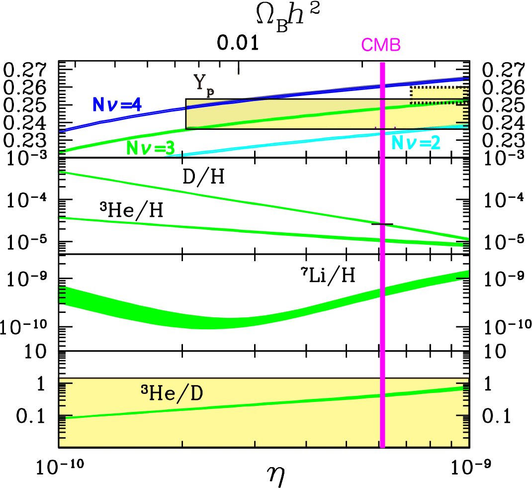
To succeed, Big Bang nucleosynthesis requires \(\frac{n_B-n_{\bar B}}{n_\gamma}\sim 10^{-9}\).
The Sakharov conditions for generating a baryon asymmetry dynamically:
- Baryon number violation (of course)
- C and CP violation (else: same rate for matter and anti-matter creation)
- Departure from thermal equilibrium (else: same abundance anti-particles, given CPT)
Not satisfied in the Standard Model.
Baryogenesis via thermal leptogenesis provides a minimal realisation, only requiring heavy right-handed neutrinos \(N_i\) (\(\rightarrow m_\nu\) via see-saw mechanism):
out-of-eq. CP-violating \(N\) decays at \(T\sim m_N\) cause lepton asymmetry
baryon asymmetry
SM sphalerons
Given R-parity, the LSP is stable and a dark matter candidate.
In a neutralino LSP scenario with \(m_{\tilde G}\sim m_\mathsf{SUSY}\):
- Thermal scattering during reheating produces gravitinos with \(\Omega^\mathsf{th}_{\tilde G} \propto T_R\)
- Thermal leptogenesis needs \(T_R \gtrsim 10^9\) GeV, to match observed baryon asymmetry
-
Due to \(M_\mathsf{Pl}\)-suppressed couplings, the gravitino easily becomes long-lived: \[\tau_{\tilde G} \sim 10^7~\mathsf{s} \left(\frac{100~\mathsf{GeV}}{m_{\tilde G}} \right)^3\]
-
Overabundant, delayed gravitino decays disrupt BBN, excluding \(T_R \gtrsim 10^5\) GeV!
So ... why not try a gravitino LSP (with neutralino NLSP)?
Gravitino trouble
Gravitino production
The gravitino relic density should match the observed \[\Omega_\mathsf{DM} h^2 = 0.1199\pm 0.0022\]
No thermal equilibrium for gravitinos in the early universe, due to superweak couplings (unless very light, but then no longer DM candidate due to Lyman-\(\alpha\))
So no standard mechanism to lower the gravitino abundance: instead, gradual build-up!
- UV-dominated freeze-in from thermal scatterings at \(T\sim T_R\) \[\Omega_{\tilde G}^{\textsf{UV}} h^2 = \left( \frac{m_{\tilde{G}}} {100 \, \textsf{GeV}} \right)\! \left(\frac{T_{\textsf{R}}}{10^{10}\,\textsf{GeV}}\right)\! \left[\,\sum_{i=1}^{3}\omega_i g_i^2 \! \left(1+\frac{M_i^2}{3m_{\tilde{G}}^2}\right) \ln\!\left(\frac{k_i}{g_i}\right) + 0.00319\, y_t^2\!\left(1+\frac{A_t^2}{3m_{\tilde{G}}^2}\right)\right]\] (accounting for 1-loop running of \(g_i, M_i, y_t, A_t\))
- IR-dominated freeze-in from decays of heaviest sparticles
- SuperWIMP contribution from decays of thermal neutralino NLSP
- (Direct inflaton decays to gravitinos)
from processes like \((g+g\rightarrow) g \rightarrow \tilde g + \tilde G \)
Gravitino production
The gravitino relic density should match the observed \[\Omega_\mathsf{DM} h^2 = 0.1199\pm 0.0022\]
No thermal equilibrium for gravitinos in the early universe, due to superweak couplings (unless very light, but then no longer DM candidate due to Lyman-\(\alpha\))
So no standard mechanism to lower the gravitino abundance: instead, gradual build-up!
- UV-dominated freeze-in from thermal scatterings at \(T\sim T_R\)
- IR-dominated freeze-in from decays of heaviest sparticles
- SuperWIMP contribution from decays of thermal neutralino NLSP \[\frac{\Omega_{\tilde G}^\mathsf{SW}h^2}{m_{\tilde G}} = \frac{\Omega_{\tilde \chi}^\mathsf{th} h^2}{m_{\tilde \chi}}\]
- (Direct inflaton decays to gravitinos)
NLSP decays
\(\tilde{\chi}_1^0 \to \tilde{G} + \gamma \)
\(\tilde{\chi}_1^0 \to \tilde{G} + Z \)
\(\tilde{\chi}_1^0 \to \tilde{G} + \gamma^* \to \tilde{G} + f \bar{f} \qquad \mathsf{for } f = u,d,s,c,b,t, e, \mu, \tau\)
\(\tilde{\chi}_1^0 \to \tilde{G} + Z^{*} \to \tilde{G} + f \bar{f} \qquad \mathsf{for } f = u,d,s,c,b,t, e, \mu, \tau\)
\(\tilde{\chi}_1^0 \to \tilde{G} + (\gamma/Z)^{*} \to \tilde{G} + f \bar{f} \qquad \mathsf{for } f = u,d,s,c,b,t, e, \mu, \tau\)
\(\tilde{\chi}_1^0 \to \tilde{G} + h^0 \to \tilde{G} + XY \qquad \mathsf{for } XY = \mu^+\mu^-,\tau^+\tau^-, c\bar c, b \bar b, g g, \gamma \gamma, Z \gamma, ZZ, W^+ W^-\)
Relevant decay channels:
Crucially, the NLSP lifetime behaves as \(\tau_{\tilde \chi} \propto M_P^2 m_{\tilde G}^2/m_{\tilde \chi}^5 \) !
BBN constraints
Lifetime/abundance limits for a generic particle decaying into \[u\bar u, b\bar b, t\bar t, gg, e^+e^-, \tau^+\tau^-, \gamma\gamma, W^+W^-\] and thus injecting energy into the primordial plasma
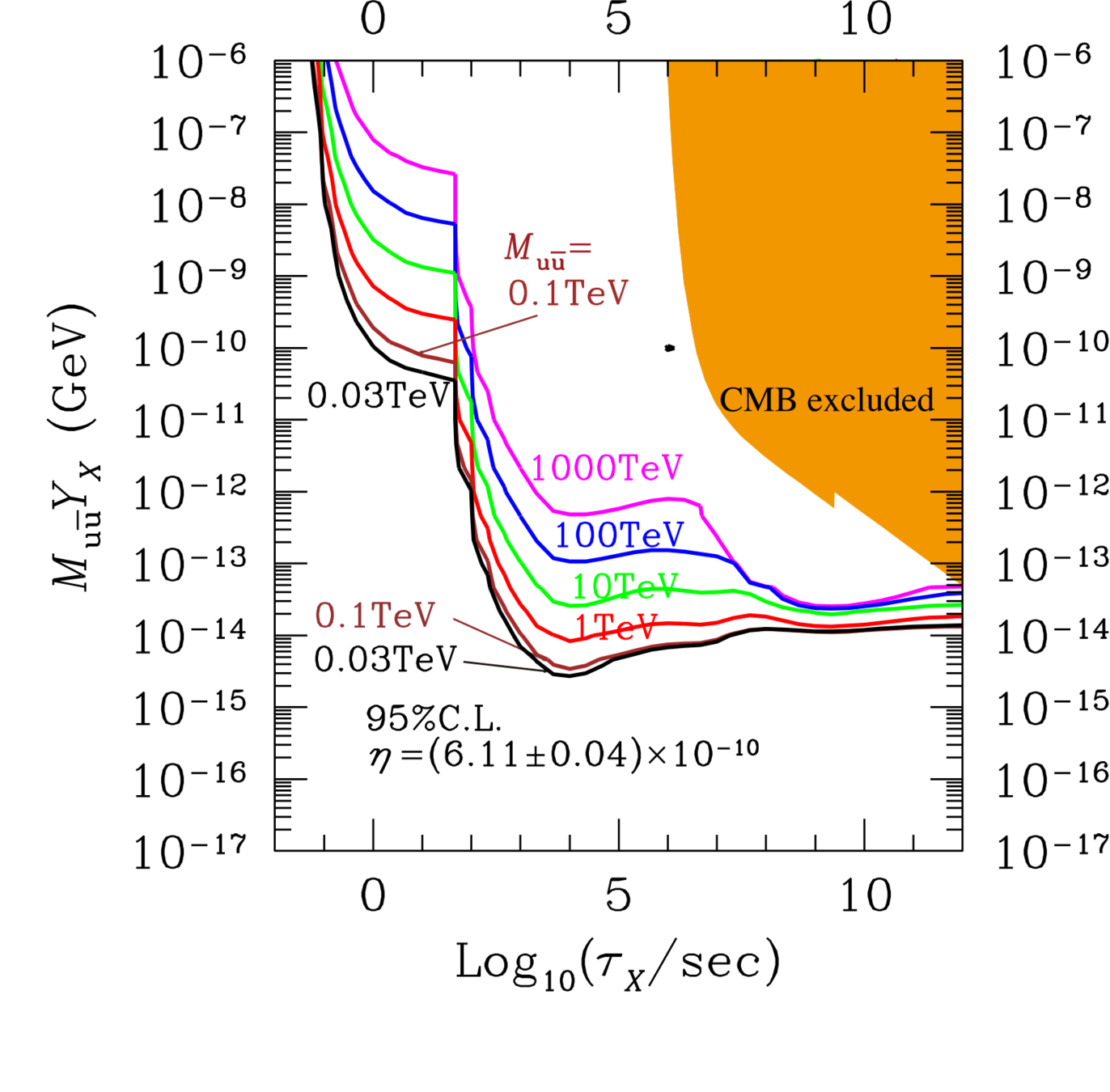
arXiv:1709.01211
p/n conversion
hadrodissociation
photodissociation
Collider constraints
Last step due to computational expense, split into 5 components:
- Quick veto with lower bound on EWino masses, upper bound on lifetimes and pass some gluino/neutralino exclusion limits from ATLAS search [1712.02332]
- Quick veto on chargino production cross-section from CMS disappearing-track search [1804.07321]
- SmodelS determines simplified model topologies and tests them against LHC limits
- CheckMATE performs event generation, detector simulation, cuts for different signal regions, and applies LHC limits
PhD Defence
By jeriek


