Parallel Numerical Methods
Presentation 1
Introduction
What's are we doing here?
Parallel Numerical Methods
What do we mean by parallel numerical methods?
Numerically solving linear systems and friends?
Takeaways for today
- What problems do we care about solving?
- Linear Algebra Review
- Software
- Parallelism
Reading
Parallel Numerical Algorithms
Editors: Keyes, David E., Sameh, Ahmed, Venkatakrishnan, V. (Eds.)
Published 1997
This book is sorta old...
Example Problem
One dimensional boundary value problem
-u^{\prime\prime}(x) + \sigma u(x) = f(x)
We want to find a function \(u(x)\) satisfying the above.
Model Problem
For \(0 < x < 1\), \(\sigma > 0\) with \(u(0)=u(1)=0\)
Example Problem
One dimensional boundary value problem
-u^{\prime\prime}(x) + \sigma u(x) = f(x)

Grid:
\(h:=\frac{1}{N}, x_j = jh, j = 0,1, \cdots N\)
\(x_0, x_1, x_2\)
\(x_j\)
\(x_N\)
Let \(f_i = f(x_i)\) and \(v_i \approx u(x_i)\), we want to recover \(v_i\)
\(\cdots\)
\(\cdots\)
\(\cdots\)
Example Problem
Taylor Series Approximation
\(u(x_{i+1}) = u(x_i) + hu^\prime(x_i) + \frac{h^2}{2}hu^{\prime\prime}(x_i) + \frac{h^3}{6}u^{\prime\prime\prime}(x_i) + O(h^4)\)
\(u(x_{i-1}) = u(x_i) - hu^\prime(x_i) + \frac{h^2}{2}hu^{\prime\prime}(x_i) - \frac{h^3}{6}u^{\prime\prime\prime}(x_i) + O(h^4)\)
Add these two together, then solve for \(u^{\prime\prime}\). This gives:
\(u^{\prime\prime}(x_i) = \frac{u(x_{i+1})-2u(x_i) + u(x_{i-1})}{h^2} + O(h^2)\)
Example Problem
Linear System
We approximate the original BVP with the finite difference scheme
\(\frac{-v_{i-1}+2v_i - v_{i+1}}{h^2} + \sigma v_i = f_i\)
With
\(v_0 = v_N = 0\)
for \(i=1,2,\cdots, N-1\)
Example Problem
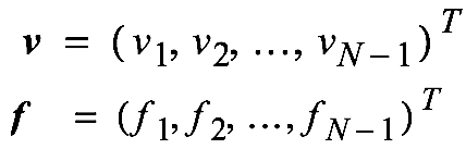
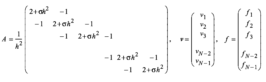
First we let:
Obtain an approximate solution by solving \(A\bm{v} = \bm{f}\) with:
Linear Algebra
We're concerned with (computationally) solving problems of the form
\(Ax=b\)
Most other problems can be restated or approximated in terms of solving a linear equation (or applying/inverting a linear operator)
Terminology
Dense Matrix: Most elements in a matrix are non-zero
Sparse Matrix: Most elements in a matrix are zero
Direct Methods: Directly solving or inverting a problem
Iterative Methods: Applying an operation multiple times until convergence to a solution
Software
Computation
How do we actually compute these things?
Basic Linear Algebra Subprograms (BLAS)
- The BLAS (Basic Linear Algebra Subprograms) are routines that provide standard building blocks for performing basic vector and matrix operations
Level 1: Scaler-vector operations
Level2: Matrix-vector operations
Level 3: Matrix-matrix operations
Linear Algebra
Let's focus on solving equations
\(Ax=b\)
So let's compute \(A^{-1}\), then find compute \(x = A^{-1}b\)?
Why is this bad?
Gaussian Elimination
\(PA=LU\)
Remember, from Linear algebra?
For a given \(N\times N\) matrix \(A\), the LU factorization of \(A\) is
Where \(L\) is a lower triangular matrix, and \(U\) is an upper triangular matrix
Why is this better than directly solving for \(A^{-1}\)?
Gaussian Elimination
\(PA=LU\)
Solving \(Ax = b\)
Since \(U\) is upper triangular, we can compute \(U^{-1}b\) in \(O(n^2)\) operations. Likewise for \(L\).
Solving \(P^TLUx = b\)
Cholesky Factorization
\(A=LL^*\)
For a given \(N\times N\) Hermatian positive definite matrix \(A\), the cholesky factorization of \(A\) is
Where \(L\) is a lower triangular matrix, and \(L^*\) is the conjugate transpose of \(L\).
QR Factorization
\(A=QR\)
For a given \(N\times N\) real matrix \(A\), the QR factorization of \(A\) is
Where \(Q\) is an orthogonal matrix, and \(R\) is an upper triangular matrix.
SVD Decomposition
\(A=U\Sigma V^*\)
For a given \(M\times N\) real matrix \(A\), the SVD decomposition of \(A\) is
Where
- \(U\) is an \(m\times m\) unitary matrix
- \(\Sigma\) is a diagonal \(m\times n\) matrix with non negative real entries
- \(V\) is an \(n \times n\) unitary matrix
Spectral Decomposition
\(A = Q\Lambda Q^{-1}\)
For a given \(N\times N\) matrix \(A\) with linearly independent eigenvectors, the spectral factorization of \(A\) is
Where \(Q\) is the matrix of eigen vectors, and \(\Lambda\) diagonal matrix of eigen values.
Computation
Cholesky
double *cholesky(double *A, int n) {
    double *L = (double*)calloc(n * n, sizeof(double));

    for (int i = 0; i < n; i++)
        for (int j = 0; j < (i+1); j++) {
            double s = 0;
            for (int k = 0; k < j; k++)
                s += L[i * n + k] * L[j * n + k];
            L[i * n + j] = (i == j) ?
                           sqrt(A[i * n + i] - s) :
                           (1.0 / L[j * n + j] * (A[i * n + j] - s));
        }

    return L;
}
Software for Computation
- Armadillo
- C++ AMP BLAS
- BLAS (Original implementation)
- uBLAS (Boost Implementation)
- LAPACK
- more...
Serial Implementations

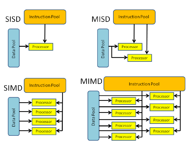
Flynn's Taxonomy
What type of architecture is your CPU? GPU?
Flynn's Taxonomy
Algorithms need to be adapted to fit the architecture of the machine they execute upon
Parallelism
Grainularity
Coarse Grain Parallelisim:
A program is split into large tasks. For example, block matrix decompositions.
Pros, cons?
What types of architectures?
Parallelism
Grainularity
Medium Grain Parallelisim:
A program is split into medium tasks. Higher throughput, but higher communication and synchronization cost.
Pros, cons?
What type of architectures?
Parallelism
Grainularity
Fine Grain Parallelisim:
A program is split into small tasks. Again, higher throughput, but higher communication and synchronization cost.
Pros, cons?
What type of architectures?
Parallelism
Grainularity
void main()
{
  switch (Processor_ID)
  {
    case 1: Compute element 1; break;
    case 2: Compute element 2; break;
    case 3: Compute element 3; break;
    .
    .
    .
    .
    case 100: Compute element 100;
              break;
  }
}
void main()
{
switch (Processor_ID)
{
case 1: Compute elements 1-4; break;
case 2: Compute elements 5-8; break;
case 3: Compute elements 9-12; break;
.
.
case 25: Compute elements 97-100;
break;
}
}void main()
{
switch (Processor_ID)
{
case 1: Compute elements 1-50;
break;
case 2: Compute elements 51-100;
break;
}
}Fine
Medium
Coarse
Parallelism
Levels of Parallelism
Instruction-level parallelism is a measure of how many of the instructions in a computer program can be executed simultaneously.
What types of architectures?
SIMD, Pipelining, OOO execution/register renaming, speculative execution...
Parallelism
Levels of Parallelism
Loop-level parallelism is a form of parallelism in software programming that is concerned with extracting parallel tasks from loops. The opportunity for loop-level parallelism often arises in computing programs where data is stored in random access data structures.
Types of architectures?
When can you do this?
Parallelism
Levels of Parallelism
Similarly, more coarse levels exist, such as subroutine and program level parallelism
Types of architectures?
Parallelism
Acheiving best performance
How do we optimize for performance (what type of granularity and level of parallelism)?
Parallelism?
Cholesky
double *cholesky(double *A, int n) {
    double *L = (double*)calloc(n * n, sizeof(double));

    for (int i = 0; i < n; i++)
        for (int j = 0; j < (i+1); j++) {
            double s = 0;
            for (int k = 0; k < j; k++)
                s += L[i * n + k] * L[j * n + k];
            L[i * n + j] = (i == j) ?
                           sqrt(A[i * n + i] - s) :
                           (1.0 / L[j * n + j] * (A[i * n + j] - s));
        }

    return L;
}
Software for Computation (GPU)
- cuBLAS
- clBLAS
- clBLAST
- ....
Parallel Numerical Methods
By Joshua Horacsek


