Parallel Numerical Methods
Iterative Methods, Conjugate Gradient, and Preconditioning
Roadmap
- Iterative Methods
- Steepest Descent and Conjugate Gradient
- GMRES
- Multigrid
Let's retread some ground to get a better feel for some of the algorithms we've investigated so far
Sparse Matrices
Saving space and time
- An \(n \times m\) matrix uses \(O(nm)\) storage
- Matrix vector multiplication costs \(O(nm)\) for \(n \times m\) matrices
- Many of problems correspond to matrices with many zero entries (or are banded/structured in some way)
- We consider these matrices to be sparse, generally we think of a matrix as sparse when the ratio of zeros to non-zeros is greater than \(\frac{1}{2}\)
- Why store zeros?
Sparse Matrices
Saving space and time
- Useful for matrices that are so large that they cannot fit in memory
- How do you store these matrices (data structures)?
\begin{bmatrix}
1 & 2 & 0 & 0 & 0 \\
0 & 1 & 0 & 0 & 0 \\
0 & 0 & 3 & 4 & 0 \\
0 & 0 & 0 & 6 & 0 \\
0 & 0 & 0 & 7 & 1
\end{bmatrix}
Sparse Matrices
Saving space and time
Set of triplets
\begin{bmatrix}
1 & 2 & 0 & 0 & 0 \\
0 & 1 & 0 & 0 & 0 \\
0 & 0 & 3 & 4 & 0 \\
0 & 0 & 0 & 6 & 0 \\
0 & 0 & 0 & 7 & 1
\end{bmatrix}
| i | j | value |
|---|---|---|
| 1 | 1 | 1 |
| 2 | 1 | 2 |
| 2 | 2 | 1 |
| 3 | 3 | 3 |
| 4 | 3 | 4 |
| 4 | 4 | 6 |
| 4 | 5 | 7 |
| 5 | 5 | 1 |
Bad for iterating over rows/columns
Fast lookup, \(O(m)\) storage
Sparse Matrices
Saving space and time
Linked Representation
\begin{bmatrix}
1 & 2 & 0 & 0 & 0 \\
0 & 1 & 0 & 0 & 0 \\
0 & 0 & 3 & 4 & 0 \\
0 & 0 & 0 & 6 & 0 \\
0 & 0 & 0 & 7 & 1
\end{bmatrix}
1
2
1
4
3
6
7
1
Sparse Matrices
Saving space and time
Compressed Sparse Row
Stores three non-zero arrays
\begin{bmatrix}
1 & 2 & 0 & 0 & 0 \\
0 & 1 & 0 & 0 & 0 \\
0 & 0 & 3 & 4 & 0 \\
0 & 0 & 0 & 6 & 0 \\
0 & 0 & 0 & 7 & 1
\end{bmatrix}
A=[1 2 1 3 4 6 7 1]
IA=[0 2 3 5 6 8]
JA=[0 1 1 2 3 3 3 4]
A = non zero columns of the matrix
IA = number of nonzero elements on the (i-1)-th row in the original matrix
JA = index of the column for an element in A
Sparse Matrices
Saving space and time
Compressed Sparse Row
A=[1 2 1 3 4 6 7 1]
IA=[0 2 3 5 6 8]
JA=[0 1 1 2 3 3 3 4]
A = non zero columns of the matrix
IA = number of nonzero elements on the (i-1)-th row in the original matrix
JA = index of the column for an element in A
def sparse_matrix_mult(n, A, IA, JA, x):
    Ax = x.copy()*0
    a_idx = 0
    for i in range(n):
        num_elements = IA[i + 1] - IA[i]
        for _ in range(num_elemnets):
            Ax[i] += x[JA[a_idx]] * A[a_idx]
            a_idx += 1
    return Ax
Sparse Matrices
Saving space and time
Related Friends
\begin{bmatrix}
1 & 2 & 0 & 0 & 0 \\
0 & 1 & 0 & 0 & 0 \\
0 & 0 & 3 & 4 & 0 \\
0 & 0 & 0 & 6 & 0 \\
0 & 0 & 0 & 7 & 1
\end{bmatrix}
- List of keys
- Compressed Sparse Columns
- Variations on CSR
Sparse Matrices
Saving space and time
- If a matrix has \(m\) non zero entries, then matrix vector multiplication is \(O(mn)\)
- Direct methods on sparse matrices?
- Factorizations can produce dense matrices, how do you store those?
Matrix Free Representations
An aside
What if you have no explicit matrix \(A\), but only a procedure that calculates \(Ax\) for a given \(x\) ?
Iterative Methods
Can massively outperform direct methods, especially when convergence is fast
Stationary
Krylov Subspace methods
Jacobi, Gauss seidel
- Iterative methods for solving linear system \(Ax = b\) begin with initial guess for solution and successively improve it until solution is as accurate as desired
- In theory, infinite number of iterations might be required to converge to exact solution
- Iteration terminates when residual \(\|b − Ax\|\), or some other measure of error is as small as desired Iterative methods are especially useful when matrix A is sparse
Non-stationary
Power Iteration
Simplest method for computing one eigenvalue-eigenvector pair is power iteration, which in effect takes successively higher powers of matrix times initial starting vector
for k in range(iterations):
	y = A.dot(x)
	x = y/y.infty_norm()
Stationary
Iterate on vector
Why do these methods work? Also, when?
\(x^{new} = Tx^{old} + c\)
T never changes
Jacobi and Gauss Siedel
\(x^*_i = \frac{b_i - \sum_{i\ne j} a_{i,j}x_j}{a_{ii}}\)
Beginning with an initial guess, both methods compute the next iterate by solving for each component of \(x\) in terms of other components of \(x\)
If D, L, and U are diagonal, strict lower triangular, and strict upper triangular portions of A, then Jacobi method can be written
\(x^* = D^{-1}(b-(L+U)x)\)
\(x^*_i = \frac{b_i - \sum_{j<i} a_{i,j}x^*_j -\sum_{j>i} a_{i,j}x_j}{a_{ii}}\)
\(x^* = (L+D)^{-1}(b-Ux)\)
Jacobi and Gauss Siedel
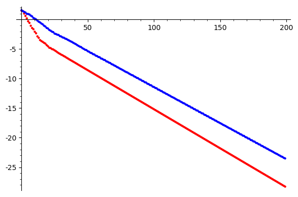
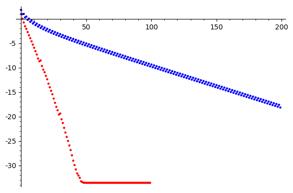
Convergence
Take a random \(100 \times 100\) matrix and solve for a random vector
\(\log \|Ax-b\|\)
Iterations
Gauss Seidel
Jacobi
Pre-preconditioners
A first introduction, sorta
Change problem slightly so that it's easier to solve.
\(x^*_i =(1-\omega)x^*_i + \omega\left(\frac{b_i - \sum_{j<i} a_{i,j}x^*_j -\sum_{j>i} a_{i,j}x_j}{a_{ii}}\right)\)
Pre-preconditioners
A first introduction, sorta
Change problem slightly so that it's easier to solve.
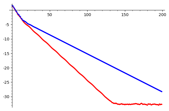
Iterations
Gauss Seidel
Gauss Seidel SOR \(\omega=0.95\)
\(\log \|Ax-b\|\)
Steepest Descent
\(\displaystyle\argmin_x \frac{1}{2}x^TAx - x^Tb\)
Obtains minimum when \(Ax=b\)
Steepest descent \(x^*=x + \alpha\nabla(\frac{1}{2}x^TAx - x^Tb)\)
\(\alpha = r^Ts/(s^TAs)\)
\(r:= b - Ax\)
If A is \(n \times n\) symmetric positive definite matrix, we minimize the quadratic form
Optimal line search parameter
Steepest Descent
def steepest_descent(A, b, max_iters = 1000):
    x = np.array([0.0] * A.shape[0])
    for _ in xrange(max_iters):
        r = b-A.dot(x)
        s = r.dot(r)
        a = s/(r.dot(A.dot(r)))
        if s < 1e-10:
            break
        x = x+a*r
    print("%d iterations" % _ )
    return x, r
Steepest Descent
Example
A = \begin{bmatrix}
2 & 0 \\
0 & 1
\end{bmatrix}
b = \begin{bmatrix}
-1 \\
5
\end{bmatrix}
Problem: Chooses the same vector more than once
Conjugate Gradient
Fixing steepest descent by choosing gradients in new, orthogonal, directions
Krylov Subspaces
\( K_n = \{b, Ab, A^2b, \cdots A^{n-1}b\}\)
General idea
Seek solutions in the space
That is, at step \(n\) look for a solution \(x_n\) such that
\(\displaystyle\min_{x_n \in K_n} \|b-Ax_n\|\)
Why find a solution in \(K_n\)?
Krylov Subspaces
General idea
\(0 = q(A)\)
\(0 = \displaystyle\sum_{i=0}^m a_iA^i\)
\(0 = a_0I + \displaystyle\sum_{i=1}^m a_iA^i\)
\(I = - \displaystyle\sum_{i=1}^m \frac{a_i}{a_0}A^i\)
\(A^{-1} = - \displaystyle\sum_{i=1}^m \frac{a_i}{a_0}A^{i-1}\)
\(A^{-1}b = - \displaystyle\sum_{i=1}^m \frac{a_i}{a_0}A^{i-1}b\)
\(x = A^{-1}b \in K_m\)
\(q(\cdot)\) is the minimal polynomial for A
\(m\) depends on the structure of the eigenvalues of \(A\)
Conjugate Gradient
Fixing SD by choosing gradients in new, unique directions

Each sucessive \(p_i\) is chosen to be orthogonal to the set \(\{p_0, \cdots, p_{i-1}\}\)
As the algorithm progresses, \(p_i\) and \(r_i\) span the same Krylov subspace.
\(x_k\)can be regarded as the projection of \(x\) on \(K_k\).
If \(m << n\), then we converge in few iterations. If we allow \(k\to n\) then we have a direct method.
Conjugate Gradient
def conjgrad(A, x, b):
    r = b - A.dot(x)
    p = r.copy()
    rsold = r.dot(r)
    e = []

    for i in range(len(b)):
        Ap = A.dot(p);
        alpha = rsold / (p.dot(Ap))
        x = x + alpha * p;
        r = r - alpha * Ap;
        rsnew = r.dot(r);
        p = r + (rsnew / rsold) * p;
        rsold = rsnew;
        e += [sqrt(rsnew)]
    return x, e
Conjugate Gradient
A = \begin{bmatrix}
2 & 0 \\
0 & 1
\end{bmatrix}
b = \begin{bmatrix}
-1 \\
5
\end{bmatrix}
Convergence
Iterations
Steepest Desc
Conj Grad
\(\log \|Ax-b\|\)
Problems
What if A isn't positive definite? What if A isn't symmetric?
Generalised Minimal Residual
\( K_n = \{b, Ab, A^2b, \cdots A^{n-1}b\}\)
Again, for an \(m\times m\) matrix \(A\) seek solutions in the space
That is, at step \(n\) look for a solution \(x_n\) such that
\(\displaystyle\min_{x_n \in K_n} \|b-Ax_n\|\)
Iteratively build up an orthogonal basis for \(K_n\) (QR decomposition) which allows us to easily solve for a given \(x_n\)
Use Arnoldi iteration to build \(Q_n\) and \(H\) such that \(AQ_n = Q_{n+1}H\) (H is Hassenberg, i.e almost upper triangular)
Arnoldi Iteration
Start with an arbitrary vector \(q_1\) with norm 1.
For k = 2, 3, …
- \(q_k = Aq_{k-1}\)
- for j in 1 to k-1
- \(h_{j,k} = q_j^*q_k\)
- \(q_k = q_k-h_{j,k}q_j\)
- \(h_{k,k-1} = \|q_k\|\)
- \(q_k = q_k/h_{k,k-1}\)
Can be built up incrementally
Generalised Minimal Residual
Use Arnoldi iteration to build \(Q_n\) and \(H\) such that \(AQ_n = Q_{n+1}H\) (H is Hassenberg, i.e almost upper triangular)
\(\|Ax_n - b\| = \|Q_{n+1}^TAx_n - Q_{n+1}^Tb\| = \|Q_{n+1}^TAQ_ny_n - Q_{n+1}^Tb\| = \|H_ny_n - \beta e_1\|\)
with \(\beta = \|b-Ax\|\)
So the algorithm is as follows, on the \(n^{th}\) iteration
- Calculate \(q_{n}\) with the Arnoldi method;
- Find the \(y_n\) which minimizes \(\|H_ny_n - \beta e_1\|\)
- Compute \(x_{n}=Q_{n}y_{n}\)
- Repeat if the residual is not yet small enough.
Since \(x\in K_n\) and \(Q_n\) is a basis for \( K_n\)
Preconditioners
Make a given problem easier
Instead of solving \(Ax = b\), we solve a related problem \(AM^{-1}y = b\) for \(y\), then compute \(x = My\)
- The matrices \(M\) and \(M^{-1}\) should be easily expressible
- The matrix \(AM^{-1}\) should be better conditioned than \(A\)
Preconditioners
Incomplete LU factorization
Since LU of sparse matrix may be dense, seek a sparse approximation to LU factorization.
Start by noting all the non-zero elements of an \(n \times n\) sparse matrix \(A\).
\(G(A) = \{(i,j) | A_{ij} \ne 0\}\)
Then choose a sparsity pattern \(S\) such that
\(S\subset \{1, \cdots, n\}^2, \ \ G(A) \subset S, \ \ \ \{(i,i) | i\in\{1\cdots n\}\} \subset S\),
A decomposition of the form \(A=LU-R\) where the following hold
- \(L\in \mathbb {R}^{n\times n}\) is a lower unitriangular matrix
- \(U\in \mathbb {R} ^{n\times n}\) is an upper triangular matrix
- \(\displaystyle L,U\) are zero outside of the sparsity pattern i.e. \(L_{ij}=U_{ij}=0\quad \forall \;(i,j)\notin S\)
- \(R\in \mathbb {R} ^{n\times n}\) is zero within the sparsity pattern i.e.\(R_{ij}=0\quad \forall \;(i,j)\in S\)
Preconditioners
Incomplete Cholesky factorization
A sparse approximation of the Cholesky factorization.
Recall the Cholesky factorization of a positive definite matrix \(A\) is \(A\) = \(LL^*\) where \(L\) is a lower triangular matrix.
Incomplete Cholesky factorization is a sparse approximation to \(L\) lower triangular matrix \(M\) that is close to \(L\). The corresponding preconditioner is \(MM^*\).
Use the algorithm for finding the exact Cholesky decomposition, except that any entry is set to zero if the corresponding entry in A is also zero.
Preconditioners
Incomplete Cholesky factorization
A sparse approximation of the Cholesky factorization.
def ichol(A):
    n = A.shape[0]
    L = np.zeros(A.shape)
    for k in range(n):
        L[k,k] = sqrt(A[k,k])
        for i in range(k+1):
            if A[i,k] != 0:
                L[i,k] = A[i,k]/L[k,k]
    return L
Preconditioners
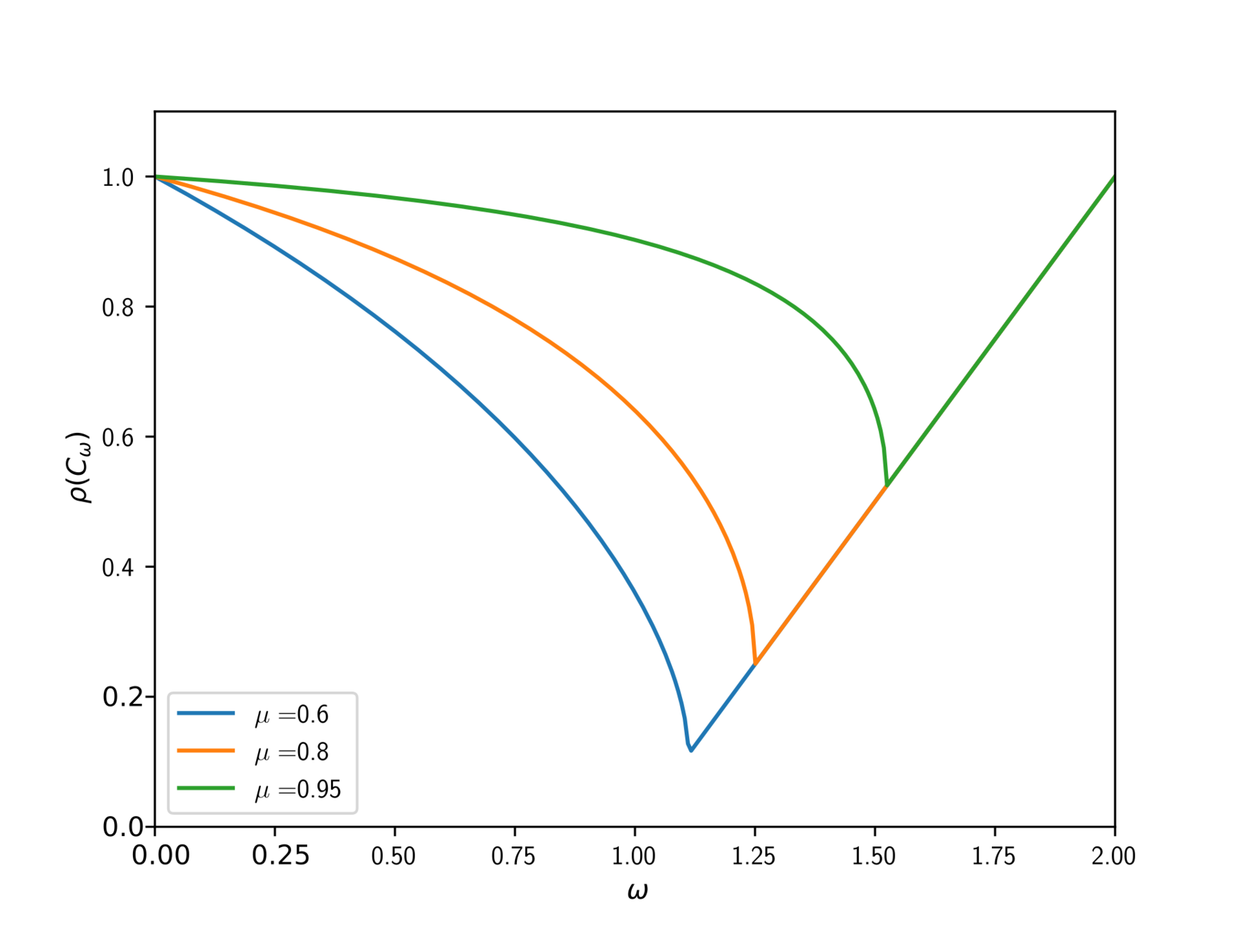
Symmetric SOR
If the original matrix can be split into diagonal, lower and upper triangular as \(A=D+L+L^T\) then the SSOR preconditioner matrix is defined as
\(M(\omega) = \frac{\omega}{2-\omega}\left(\frac{1}{\omega} D + L\right)D^{-1}\left(\frac{1}{\omega} D + L\right)^T\)
What makes a good preconditioner?
Multigrid
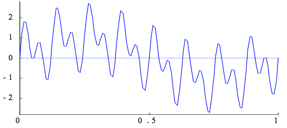
Many iterative methods have the smoothing property where oscillatory modes of the error are eliminated effectively, but smooth modes are damped slowly.
So we transform the problem such that we forcibly dampen lower frequency error modes. I.e we solve a similar problem on coarser grids, then use that as an estimate for our initial guess
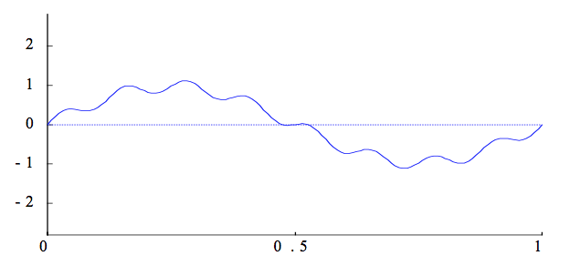
After a few iterations
Example Problem
One dimensional boundary value problem
-u^{\prime\prime}(x) + \sigma u(x) = f(x)
We want to find a function \(u(x)\) satisfying the above.
Model Problem
For \(0 < x < 1\), \(\sigma > 0\) with \(u(0)=u(1)=0\)
Example Problem
One dimensional boundary value problem
-u^{\prime\prime}(x) + \sigma u(x) = f(x)

Grid:
\(h:=\frac{1}{N}, x_j = jh, j = 0,1, \cdots N\)
\(x_0, x_1, x_2\)
\(x_j\)
\(x_N\)
Let \(f_i = f(x_i)\) and \(v_i \approx u(x_i)\), we want to recover \(v_i\)
\(\cdots\)
\(\cdots\)
\(\cdots\)
\(x_0, x_1, x_2\)
\(x_j\)
\(x_{N/2}\)
\(\cdots\)
\(\cdots\)

\(\Omega_h\)
\(\Omega_{2h}\)
Residual Correction
If we call \(e = \tilde{x} - x \), that is, \(e\) is the error between an approximation and ground truth, then \(A(\tilde{x} + e) = b\)
It follows that \(Ae = r\), so solve for \(e\) approximately, then add that to \(\tilde{x}\).
Coarse grid correction
Given an approximation to \(x\), calculate the residual \(r\) then project onto a coarser grid (restriction).
Solve for \(e\) on coarser grid, with a coarser approximate operator to \(A\).
Interpolate \(e\) on the finer grid, and perform residual correction (prolongation).
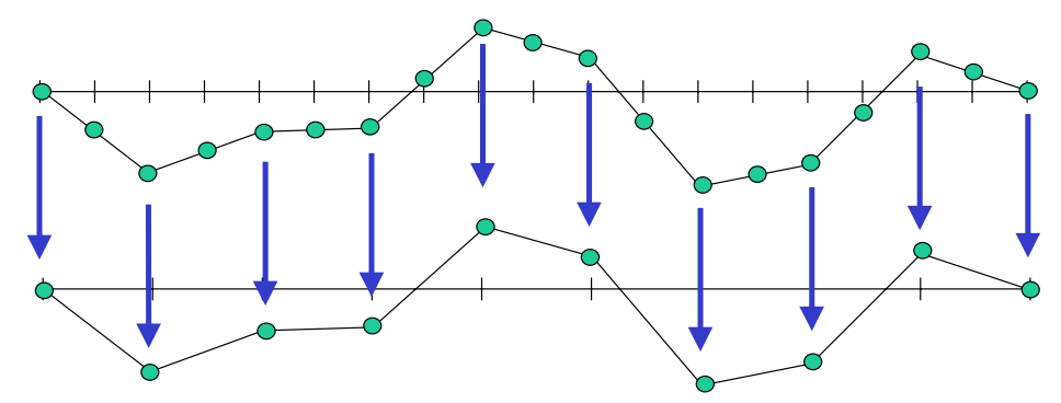
Restriction
Given an approximation to \(x\), calculate the residual \(r\) then project onto a coarser grid (restriction).
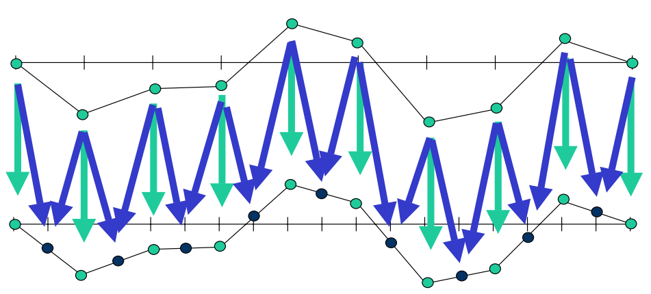
Prolongation
Interpolate \(e\) on the finer grid, and perform residual correction (prolongation).
Parallel Numerical Methods: Iterative Methods & Preconditioners
By Joshua Horacsek


