Parallel Numerical Methods
Multigrid
Roadmap
- Example problem
- Iterative Methods
- Residual Correction
- Coarse grids
- Multigrid
This topic brings together many elements we've already talked about
Example Problem
One dimensional boundary value problem
-u^{\prime\prime}(x) + \sigma u(x) = f(x)
We want to find a function \(u(x)\) satisfying the above.
Model Problem
For \(0 < x < 1\), \(\sigma > 0\) with \(u(0)=u(1)=0\)
Example Problem
One dimensional boundary value problem
-u^{\prime\prime}(x) + \sigma u(x) = f(x)
We want to find a function \(u(x)\) satisfying the above.
Model Problem
For \(0 < x < 1\), \(\sigma > 0\) with \(u(0)=u(1)=0\)
Example Problem
One dimensional boundary value problem
-u^{\prime\prime}(x) + \sigma u(x) = f(x)

Grid:
\(h:=\frac{1}{N}, x_j = jh, j = 0,1, \cdots N\)
\(x_0, x_1, x_2\)
\(x_j\)
\(x_N\)
Let \(f_i = f(x_i)\) and \(v_i \approx u(x_i)\), we want to recover \(v_i\)
\(\cdots\)
\(\cdots\)
\(\cdots\)
Example Problem
Taylor Series Approximation
\(u(x_{i+1}) = u(x_i) + hu^\prime(x_i) + \frac{h^2}{2}hu^{\prime\prime}(x_i) + \frac{h^3}{6}u^{\prime\prime\prime}(x_i) + O(h^4)\)
\(u(x_{i-1}) = u(x_i) - hu^\prime(x_i) + \frac{h^2}{2}hu^{\prime\prime}(x_i) - \frac{h^3}{6}u^{\prime\prime\prime}(x_i) + O(h^4)\)
Add these two together, then solve for \(u^{\prime\prime}\). This gives:
\(u^{\prime\prime}(x_i) = \frac{u(x_{i+1})-2u(x_i) + u(x_{i-1})}{h^2} + O(h^2)\)
Example Problem
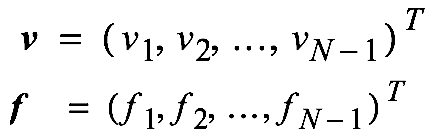
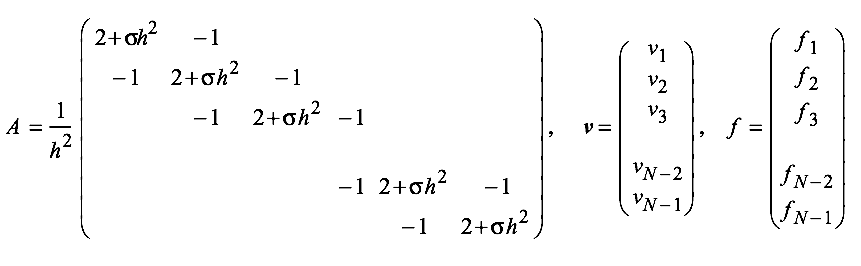
First we let:
Obtain an approximate solution by solving \(A\bm{v} = \bm{f}\) with:
Residual Correction
If we let \(e = \tilde{x} - x \), that is, \(e\) is the error between an approximation \(\tilde{x}\) and ground truth, then \(A(\tilde{x} + e) = b\)
Let \(r = b-A\tilde{x}\). It follows that \(Ae = r\), so solve for \(e\) approximately, then add that to \(\tilde{x}\).
I.e Compute \(r\), then find \(e = A^{-1}r\) and compute \(x = \tilde{x} - r\)
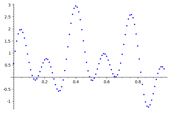
Experiment
Let's try this on our model problem
\(v_j=\sin(k \pi j/N) \)
Choose \(0<k<N\)
\(f_j = 0\)
This problem has a trivial solution, but is numerically interesting
\(\sigma = 0.1\)
Error Reduction?
Let's try this on our model problem
We'll take these as inital guesses
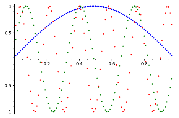
k = 1
k = 6
k = 11
Jacobi and Gauss Siedel
\(x^*_i = \frac{b_i - \sum_{i\ne j} a_{i,j}x_j}{a_{ii}}\)
Beginning with an initial guess, both methods compute the next iterate by solving for each component of \(x\) in terms of other components of \(x\)
If D, L, and U are diagonal, strict lower triangular, and strict upper triangular portions of A, then Jacobi method can be written
\(x^* = D^{-1}(b-(L+U)x)\)
\(x^*_i = \frac{b_i - \sum_{j<i} a_{i,j}x^*_j -\sum_{j>i} a_{i,j}x_j}{a_{ii}}\)
\(x^* = (L+D)^{-1}(b-Ux)\)
Jacobi SOR
\(x^*_i = (1-\omega)x_i + \omega\frac{b_i - \sum_{i\ne j} a_{i,j}x_j}{a_{ii}}\)
Beginning with an initial guess, both methods compute the next iterate by solving for each component of \(x\) in terms of other components of \(x\)
Error Reduction?
Vector Components
Error
k = 1
k = 6
k = 11
Moral?
Vector Components
Error
After a few iterations \(\omega=\frac{2}{3}\)
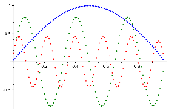
Error Reduction?
Inital Guess (sum of our last inital guesses)
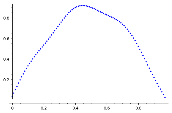
After 300 iterations
Jacobi is good at removing high-frequency error, but low frequency remains
Error
Error
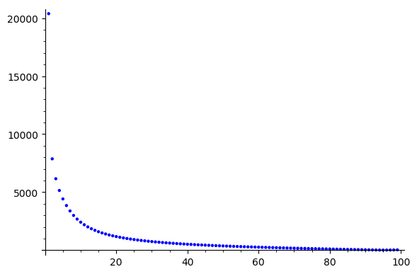
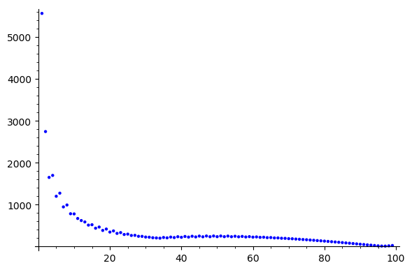
Error Reduction?
Iterations
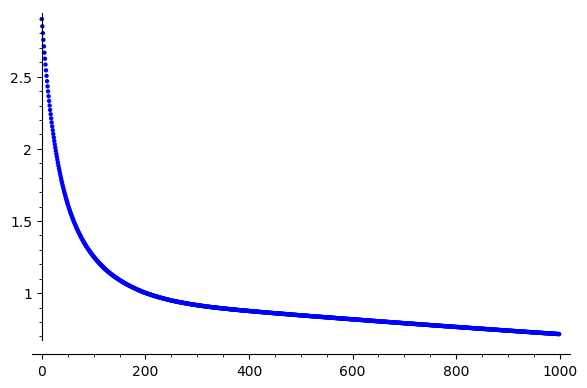
\(\|e\|_\infty\)
Error reduction stalls, why?
Error Reduction?
Jacobi
Jacobi SOR
Error Reduction?
Jacobi
Gauss Siedel
Coarse Grids
\(x_0, x_1, x_2\)
\(x_j\)
\(x_N\)
\(\cdots\)
\(\cdots\)
\(\cdots\)
\(x_0, x_1, x_2\)
\(x_j\)
\(x_{N/2}\)
\(\cdots\)
\(\cdots\)

\(\Omega_h\)
\(\Omega_{2h}\)
\(\Omega_{2^kh}\)
\(\vdots\)
\(\vdots\)
\(x_0\)
\(x_{N/2^k}\)
\(\cdots\)
Move computation to coarser grids
Why?
Coarse Grids
\(x_0, x_1, x_2\)
\(x_j\)
\(x_N\)
\(\cdots\)
\(\cdots\)
\(\cdots\)
\(x_0, x_1, x_2\)
\(x_j\)
\(x_{N/2}\)
\(\cdots\)
\(\cdots\)
\(\Omega_h\)
\(\Omega_{2h}\)
Move computation to coarser grids
Observation:
From wavelet theory, if we filter then downsample, we split the frequency content between high and low bands.
On the coarse grid, we have less work, and the low-frequency content that was on our original grid is now higher frequency
Nested Iteration
A general idea
- Solve equation on coarsest grid
- Refine grid
- If not on finest grid, go to 1
Problems?
How do we solve the problem on coarser grids. I.e. what is our operator? What if, at different levels of refinement, we introduce smooth error?
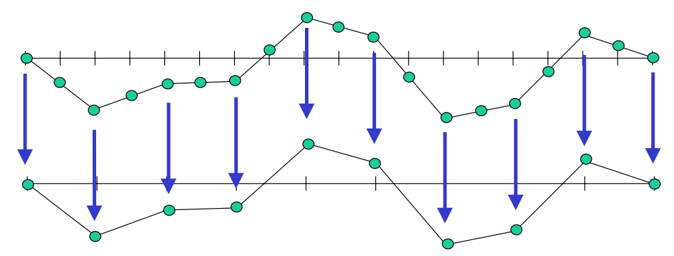
Prolongation
Interpolate \(e\) on the finer grid, and perform residual correction (prolongation).
Prolongation
Connection to wavelets?
Again, upsampling and filtering (linear b-spline)
This is a linear operator from the coarser grid onto the finer grid, we'll call it \(\Uparrow^{h}_{2h} : \Omega^{2h} \to \Omega^h\)
Prolongation
If we're solving \(Ax=b\) on a coarser grid, what's the linear operator \(A\) on that grid?
If we know that, then we just start with an initial guess vector of 0, use an iterative method for a few iterations, then "prolong" on to a finer grid.
We'll come back to this in a bit
Coarse Grid Correction
What about the high frequency error?
Iterating on a coarse grid can correct high frequency errors, the steps are
- Solve the problem on the fine grid
- Move to a coarser grid
- Solve the problem on the coarser grid
- Use this solution to update fine grid
Similar issues to nested iteration. How do you move to a coarser grid, what's the operator there?
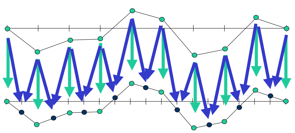
Restriction
Given an approximation to \(x\), calculate the residual \(r\) then project onto a coarser grid (restriction).
Restriction
Given an approximation to \(x\), calculate the residual \(r\) then project onto a coarser grid (restriction).
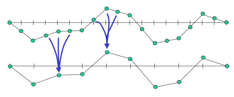
Restriction
Connection to wavelets?
Filtering and downsampling
This is a linear operator from the finer grid onto the coarser grid, we'll call it \(\Downarrow^{h}_{2h} : \Omega^{h} \to \Omega^{2h}\)
Restriction
If we're solving \(Ax=b\) on a finer grid, what's the linear operator \(A\) on that grid?
If we know that, then we just start with an initial guess vector of 0, use an iterative method for a few iterations, then "restrict" to a coarser grid, solve for a few iterations, then project back up.
Linear operator levels
Let \(A_h\) be the operator of interest on a grid \(\Omega^h\)
\(A_{2h} = \Downarrow^{h}_{2h} A_h \Uparrow^{h}_{2h}\)
By noting the problem that must be solved on the coarser grids we can obtain the following relationship
Multigrid
Multigrid is a combination of these idea
- Nested iteration fixes smooth error
- Coarse grid correction fixes oscillatory error
Correction scheme
- Iteratively solve \(A_hx=b\) on grid \(\Omega^h\) for a few iterations, with inital guess \(v\)
- Compute \(r = b-A_hx\)
- Compute \(r^\prime = \Downarrow^{h}_{2h}r \)
- Solve \(A_{2h}e = r^\prime\) for \(e\) on \(\Omega^{2h}\)
- Correct guess \(v=v + \Uparrow^{h}_{2h}e\)
- Iterate \(A_hx=b\) on grid \(\Omega^h\) with guess \(v\) from previous step
Solve equation in step 4 recursively.
Coarse grid correction
Iterate \(A_h\tilde{x} = b\)
Compute \(r = b -A_h\tilde{x} \)
Restrict \(r^\prime = \Downarrow^h_{2h}r\)
Solve \(A_{2h}e =r^\prime\)
Prolong \(e= \Uparrow^h_{2h}e\)
Update \(\tilde{x} =\tilde{x} + e\)
Iterate \(A_h\tilde{x} = b\)
Storage requirement: \(r, b, \tilde{x}\)
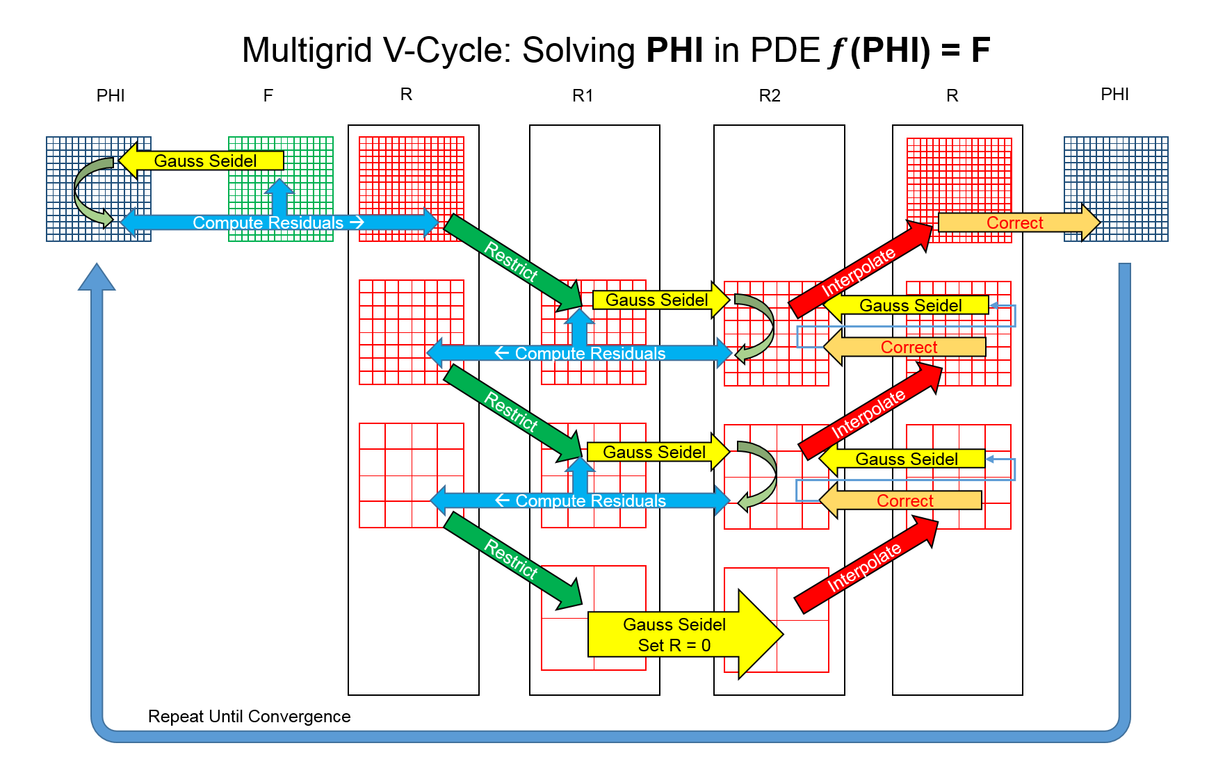
V-cycle
Finest Grid
Coarsest Grid
Finest Grid
Storage requirements?
Computation requirements?
Full Multigrid
Coarsest Grid
Finest Grid
Multigrid
Final Project
Parallel sparse GMRES solver:
- Currently implemented in CUDA (cuSPARSE and cuBLAS) and Eigen
- Hessenberg matrix and the orthogonal basis for the Krylov subspace are dense, so use cuBLAS to compute them
- However, implementations already exist (in ViennaCL and MAGMA)
Pulled matrices from the matrix market to test for correctness. Not quite "big data" but large enough to be non-trivial
Final Project
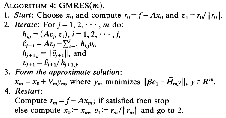
Low Syncronization GMRES algorithms
Final Project
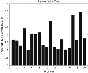
A simple strategy for varying the restart parameter in GMRES(m)
Final Project
A simple strategy for varying the restart parameter in GMRES(m)
Final Project
Multigrid on non-Cartesian lattices
- Choose a problem (Perhaps CFD problem)
- Discretize over BCC or FCC lattice
- Implement MG
- What are the appropriate prolongation/restriction operators?
- Are there different convergence properties?
Ideas?
References
- Multigrid tutorial - http://www.math.ust.hk/~mamu/courses/531/tutorial_with_corrections.pdf and https://www.math.ust.hk/~mawang/teaching/math532/mgtut.pdf
- Multigrid: Wikipedia - https://en.wikipedia.org/wiki/Multigrid_method
-
Mathematical Methods for Engineers II: Multigrid Methods - https://ocw.mit.edu/courses/mathematics/18-086-mathematical-methods-for-engineers-ii-spring-2006/readings/am63.pdf
Parallel Numerical Methods: Multigrid and Final Project Ideas
By Joshua Horacsek


