Poisson Surface Reconstruction on non-Cartesian lattices
Joshua Horacsek, Usman Alim, Torsen Möller
Surface reconstruction
(Calakli 2011)
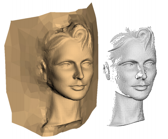
Given a set of points, find a triangular mesh that "best" fits these points
- Interpolating?
- Noisy data?
- Uniform data?
- What assumptions about the data are made?
Some review...
A Brief Survey
- Surface Reconstruction From Unorganized Points (Hoppe 1992)
- Smoothed Signed Distance Field (Calaki 2011)
-
Reconstruction and representation of 3D objects with radial basis functions (Carr 2001)
-
Hermite radial basis functions Implicits (Macedo 2011)
-
Floating scale surface reconstruction (Fuhrmann 2014)
-
Reconstruction of solid models from oriented point sets (Kahzdan 2005)
-
Poisson Surface Reconstruction (Kahzdan 2006, 2014)
-
Surface Reconstruction from Oriented Point Cloud Using a Box-Spline on the BCC Lattice (Kim 2015)
Poisson Surface Reconstruction
If you can construct a "good" approximation for V, then you can obtain an indicator function via solving the poisson problem
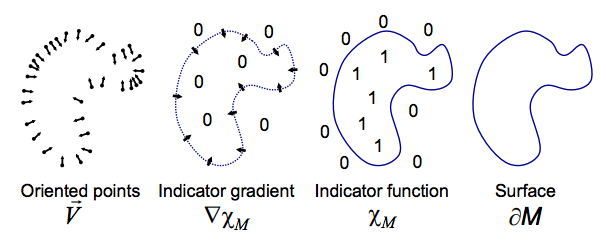
\Delta \chi_M = \nabla \cdot V
Consider a model M
(Kazhdan 2006)
Poisson Surface Reconstruction
If we N have oriented points, denoted by the set
(Kazhdan 2006)
S = \{(p_1, n_1), (p_2, n_2), \cdots (p_N, n_N)\}
Then the we have
\displaystyle\nabla(\chi_M * F)(x) \approx \sum_{(p,n) \in S}|P_s|F(x - p)\cdot n.
So we define
V(x) := \sum_{(p,n) \in S}|P_s|F(x - p)\cdot n
Poisson Surface Reconstruction
This is then distributed over nodes of an oct-tree, then a multi-grid conjugate gradient solver is used to invert the problem.
(Kazhdan 2006)
Problems?
- Cartesian structure
- Smoothing in vector field equation
What if we choose a non Cartesian lattice?
A 30% reduction in samples can be achieved on the BCC lattice v.s. the CC lattice
Poisson Surface Reconstruction
A 30% reduction in samples can be achieved on the BCC lattice v.s. the CC lattice.
The Body Centred Cubic lattice
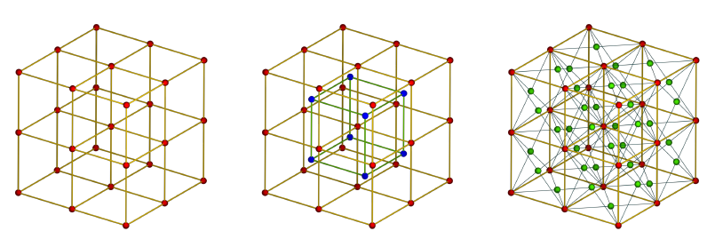
Cartesian
Body Centered Cubic (BCC)
Face Centered Cubic (FCC)
Optimal Lattices
Think about the Fourier transform of a sampled signal
(Entezari 2009)
A sampling of a function is equivalent to a periodization about its dual lattice.
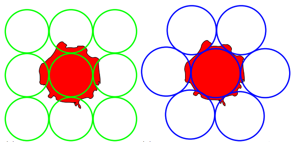
Optimal Lattices
Cartesian
Body Centered Cubic (BCC)
Face Centered Cubic (FCC)
FCC is the optimal sphere packing lattice, so the BCC lattice is the optimal sampling lattice.
A 30% reduction in samples can be achieved on the BCC lattice v.s. the CC lattice
Optimal Lattices
The BCC lattice is generated by the matrix
Pipeline
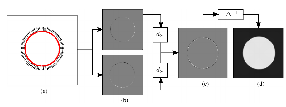
- a) Start with the input pointset
- b) Construct an approximation for V(x)
- c) Approximate the divergence of V(x)
- d) Invert the Poisson problem
Then extract the iso surface
Constructing V(x)
We want to take the initial point-set and resample it onto a regular grid. But we want to respect the geometry of that grid.
Constructing V(x)
We define V(x) as
V(x) := L \cdot [v_1(x) \ v_2(x) \ v_3(x)]^T
Where L is a basis for
Using a minimization procedure, we find the functions that minimize
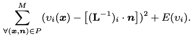
For every component.
\mathbb{R}^3
Function Spaces
In general the form we use to define a function space is
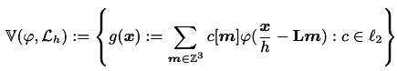
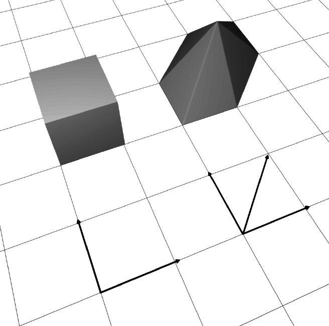
Box Splines
Box splines are piecewise polynomial functions that we use to span these spaces (think multivariate b-splines)
Defined by an s by n direction matrix
X := \begin{bmatrix}
| & | & \ & | \\
\xi_1 & \xi_2 & \cdots & \xi_n \\
| & | & \ & |
\end{bmatrix}

Box Splines
Example
Irregular sampling
If we have scattered data, how do we extrapolate those data?
But really, how do we approximate V(x)?
Intuitively, what do we want?
- The approximation should try to interpolate the data, perhaps not perfectly
- The approximation should be compact, so as to not over smooth the data
- The approximation should still be smooth
Irregular sampling
Suppose we look for some function
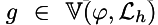
That minimizes the function
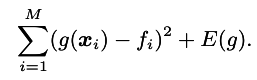
We get interpolation, but what about this energy function E(g)?
Irregular sampling
\langle f,g\rangle := \int f(x) g(x) \ dx
Define
\langle f, g \rangle_{BL^2} := \displaystyle\sum_{|p|=2} \frac{n!}{p!} \langle D^pf, D^pg \rangle
Inner Product
Beppo-Levi Inner Product
We have the induced norms
||f||^2 := \langle f,f\rangle
||f||^2_{BL^2} := \langle f, f \rangle_{BL^2}
Forces coefficients to be zero
(Volumetric) Smoothness
Our energy term is then
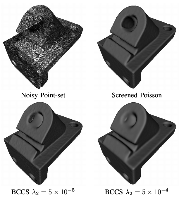
E(g) = \lambda_1 ||g|| + \lambda_2 ||g||_{BL^2}
Divergence of V(x)
We can define filters that respect the geometry and approximation order of the space
Divergence of V(x)
Notice that
\nabla \cdot V(x) = \nabla L \cdot [v_1(x) \ v_2(x) \ v_3(x)]^T
So we can use directional derivatives to take the divergence of V. This is a more natural approach on the BCC lattice
= [\nabla b_1 \ \nabla b_2 \ \nabla b_3 ] \cdot [v_1(x) \ v_2(x) \ v_3(x)]^T
= D_{b_1} v_1(x) + D_{b_2} v_2(x) + D_{b_3} v_3(x)
Use the digital filter
d[n] := [\frac{-1}{12} \ \frac{2}{3} \ 0 \ \frac{-2}{3} \frac{1}{12}]
Taking the Divergence of V(x)
We can also do reconstructions on shifted bases, and reconstruct from an overdetermined basis....
Inverse Poisson
Consider this as a "resampling" from the regular grid on to another regular grid, and a filtering that solves the Poisson problem.
We want to respect the approximation order of the space.
Error Analysis
Fourier error kernel
It's possible to quantify the approximation error for a function given its sampling and reconstruction scheme
\varphi = \text{ basis function}
\bar\varphi = \text{ analysis basis}
\dot\varphi = \text{ dual basis}
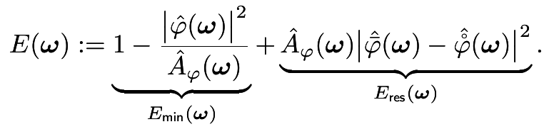
A_\varphi = \text{ auto correlation of generating function}
Error Analysis
Extension to linear operators, residual error becomes
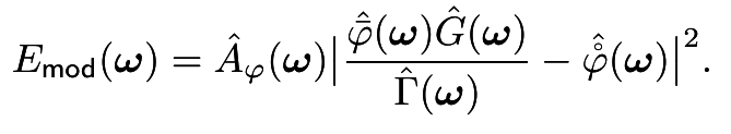
Here we have
\hat{G}(\omega) = \text{ digital filter}
\hat{\Gamma}(\omega) = \text{ linear operator}
We can use this to discretize the Laplacian and find an inverse filter that respects the approximation power of the space.
Error Analysis
This leads to the proposition
\text{For point sampled functions, let the digital filter } \hat{L}(\omega) \text{ be given by the }
\text{combined filter } \hat{L}(\omega) = \hat{P}_\varphi(\omega)\hat{\Lambda}(\omega), \text{ where } \Lambda \text{ satisfies }
\hat{\Lambda}(\omega) = -4\pi^2||\omega||^2 + O(||\omega||^{k+2})
\text{where } \hat{P}_\varphi \text{ is the interpolation prefilter for } \varphi \text{ on a given lattice. Then the }
\text{combined inverse filter } \hat{L^{-1}} \text{ provides a k-th order asymptotically optimal }
\text{discretization of the inverse Laplacian } \Delta^{-1}.
Proposition:
Inverse Poisson
We just need an appropriate filter, then we can transform the approximation into the Fourier domain, apply the filter, and take the inverse transform.
Extracting the Iso-surface
Find a level-set
c := \frac{1}{N}\displaystyle\sum_{(p,n)\in S} \chi(p).
Use an unambiguous marching cubes algorithm at a high resolution to extract
\chi(x) = c
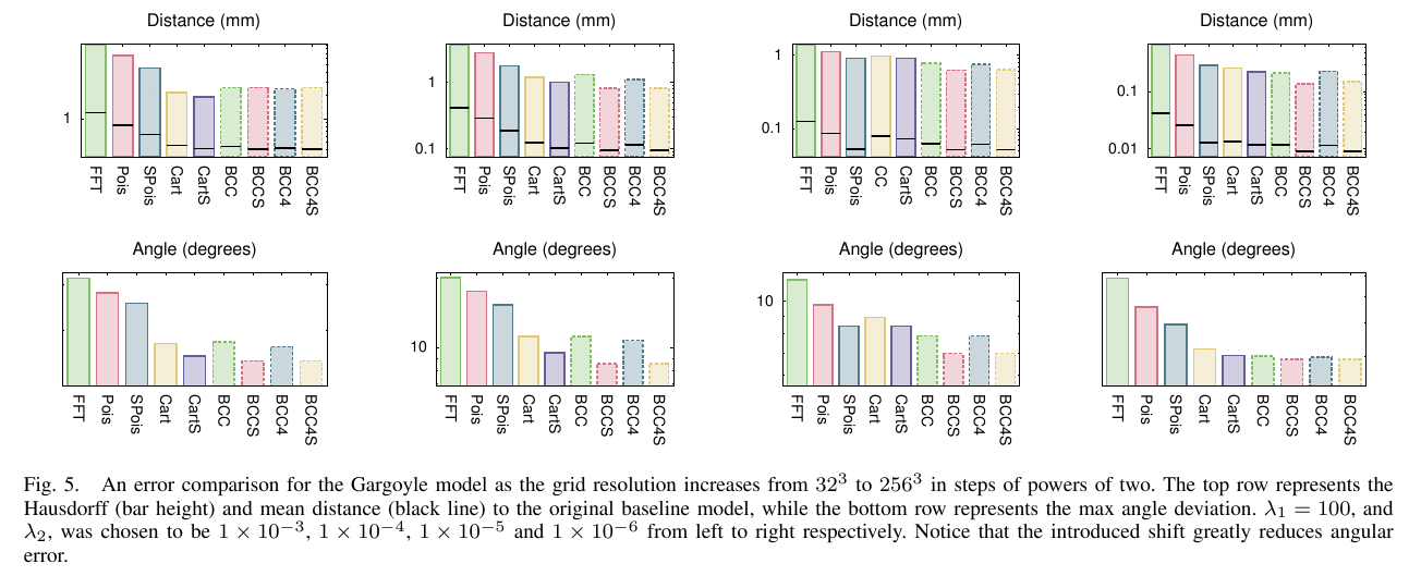
Experiments
Use Surface Reconstruction Benchmark (Berger 2013) to compare between BCC and CC (plus FFT and Poisson Methods). Grid size is chosen carefully...
- Fixing the model and alternating grid size
- Fix grid size and alternate the model
Look at noisy datasets
Try to get some quantitate results by
Look at average distance from the original model, and angular deviation
Experiments
CC lattice
X :=
\begin{bmatrix}
1 & 1 & 1 & 0 & 0 & 0 & 0 & 0 & 0 \\
0 & 0 & 0 & 1 & 1 & 1 & 0 & 0 & 0 \\
0 & 0 & 0 & 0 & 0 & 0 & 1 & 1 & 1
\end{bmatrix}
\varphi(x) = M_X(x - \frac{1}{2}\sum^9_{i=1}\xi_i)
Function Space:
Basis:
L :=
\begin{bmatrix}
1 & 0 & 0 \\
0 & 1 & 0 \\
0 & 0 & 1
\end{bmatrix}
Inverse Laplacian Filter:
\hat\Lambda(\omega) := \hat\Lambda_1(\omega_1) + \hat\Lambda_1(\omega_2) + \hat\Lambda_1(\omega_3)
\hat\Lambda_1(\omega) := \frac{2}{3}(-7 + \cos(2\pi\omega))\sin^2(\pi\omega)
Experiments
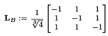
BCC lattice
X :=
\begin{bmatrix}
-1 & -1 & 1 & 1 & 1 & 1 & -1 & -1 \\
1 & 1 & -1 & -1 & 1 & 1 & -1 & -1 \\
1 & 1 & 1 & 1 & -1 & -1 & -1 & -1
\end{bmatrix}
\varphi(x) = M_X(x)
Function Space:
Basis:
L :=
\begin{bmatrix}
-1 & 1 & 1 \\
1 & -1 & 1 \\
1 & 1 & -1
\end{bmatrix}
Inverse Laplacian Filter:
\hat\Lambda(\omega) := \sum^n_{i=1}\hat\Lambda_1(\theta_i\cdot\omega)
Results
Fixed model
Results
Variable model
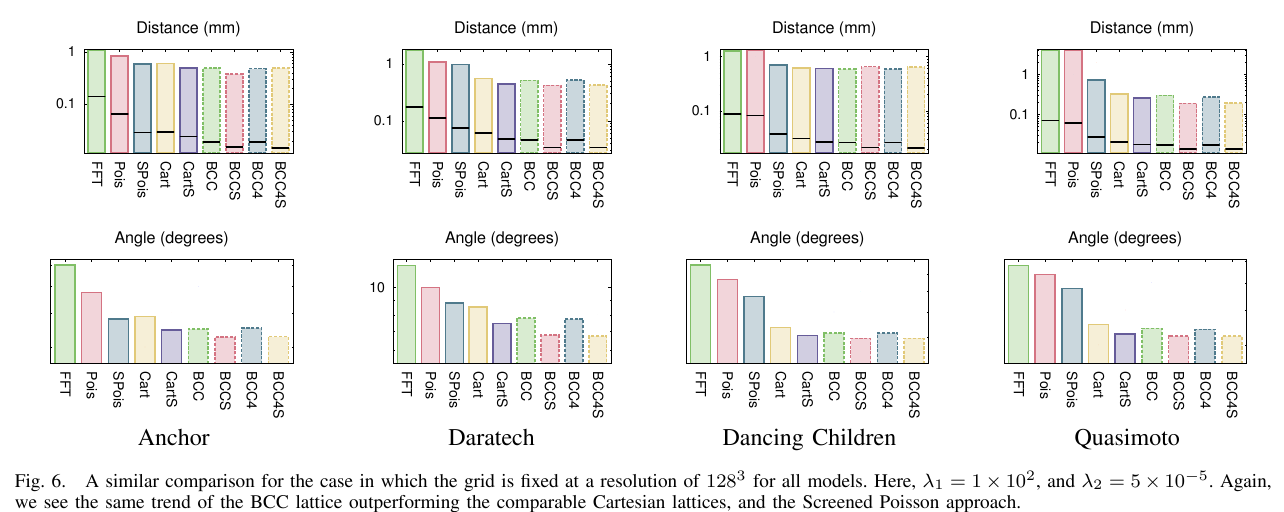
Results
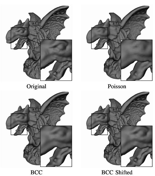
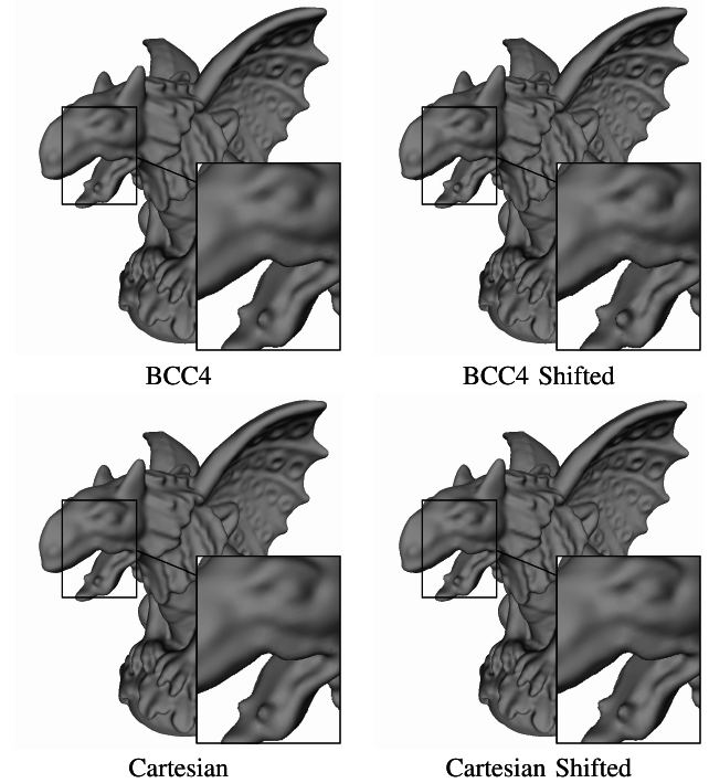
Results
Conclusion
Decent reconstructions, some problems
- Regular grid = huge memory requirement
- Optimization problem is sparse, but still very computationally intensive
- Uniform point sampling
Thanks!
Poisson Surface Recon
By Joshua Horacsek


