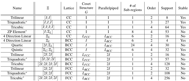
SISL and Fast Spline Evaluation
J. Horacsek
Nov 17th, 2017
Motivation
For scalar vis, we often care about evaluating functions of the form
f(x) = \displaystyle\sum_{n\in L\mathbb{Z}^3}c_n \ \varphi(x-n)
And we want to do this quickly; this is required for interactive visualization of datasets
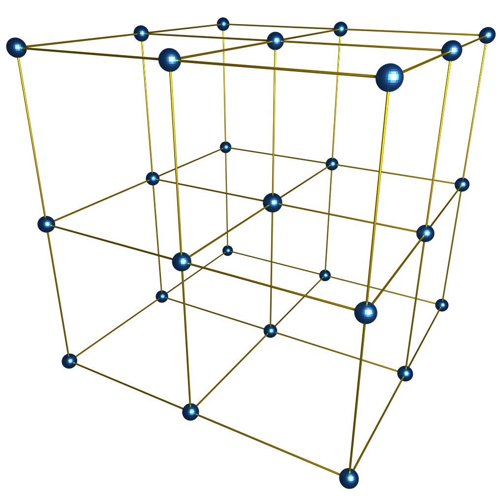
Sampling Lattices
Cartesian Lattice
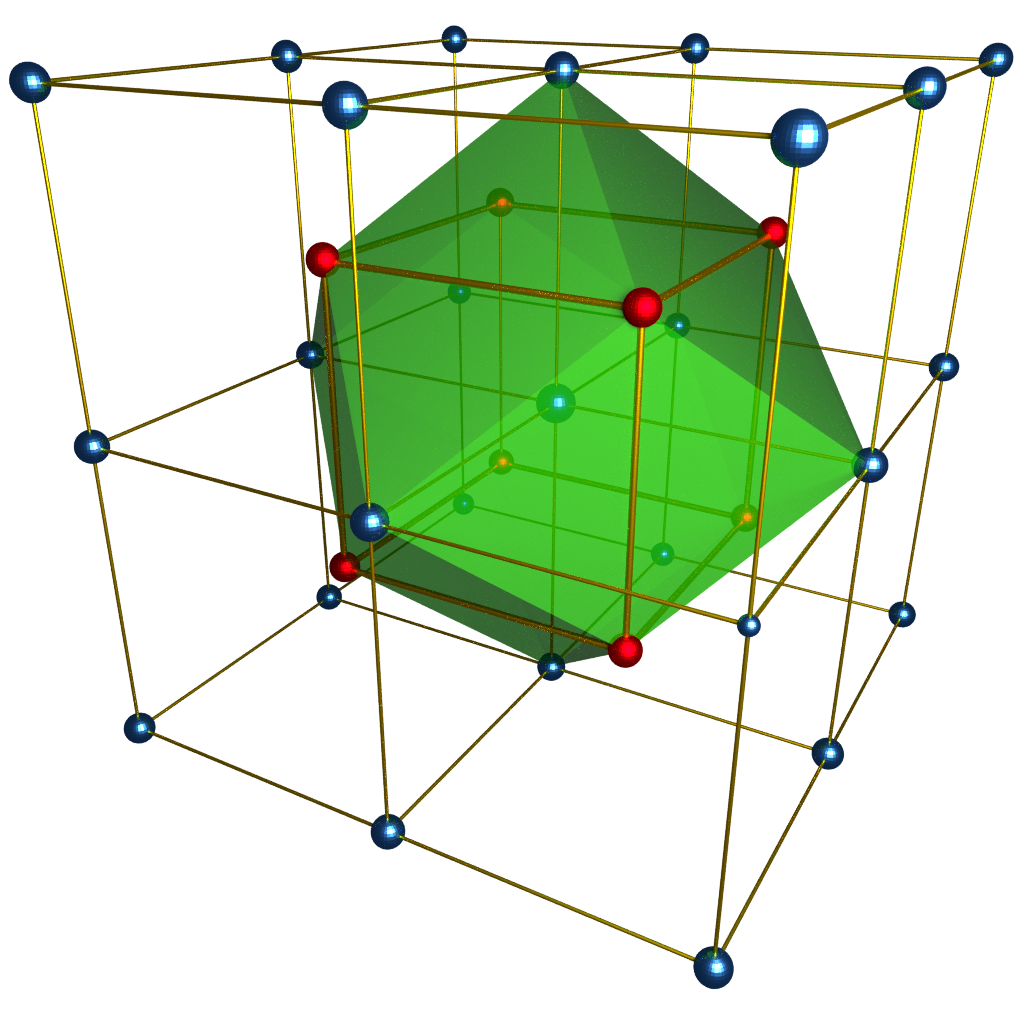
Body Centered Cubic Lattice
\displaystyle\sum_{n\in L\mathbb{Z}^3}c_n \ \varphi(x-n)
L controls the point distribution
Box Splines
Multivariate extension to B-splines
- Compact
- Smooth
- Piecewise polynomials
\Xi = \begin{bmatrix}
| & | & \ & | \\
\xi_1 & \xi_2 & ... & \xi_n \\
| & | & \ & |
\end{bmatrix}
Start with a direction matrix
\xi_i \in \mathbb{R}^s
Box Splines
Convolutional, recursive definition
M_\Xi(x) = \displaystyle\int_0^1M_{\Xi\backslash\xi}(x - t\xi) dt \text{ \ with \ } M_{[ \ ]}(x) := \delta(x)
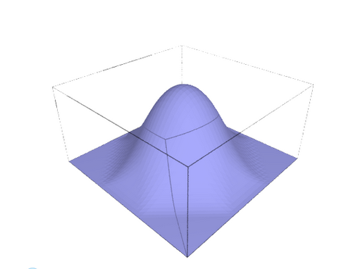
In one dimension, this looks sort of like
Box Splines
\Xi = \begin{bmatrix}
1 & 0 & 1 \\
0& 1 & 1
\end{bmatrix}
Box Splines
\Xi = \begin{bmatrix}
1 & 0 & 1 & -1 \\
0& 1 & 1 & 1
\end{bmatrix}
Box Splines
Multivariate extension to B-splines
- Compact
- Smooth
- Piecewise polynomials
Box Splines
We have an explicit form of evaluation
M_\Xi(x) = \displaystyle\sum_{(\gamma,p)\in S_\Xi} \sum_{(\lambda, \alpha) \in P_{n-s}} \gamma\lambda |\det\Xi_\alpha|{{[\![ (\Xi_\alpha^{-1}x) - p ]\!]}_{+}}^{\mu_\alpha - 1}.
(this is just a piecewise polynomial....)
But we still have the problem of evaluating
f(x) = \displaystyle\sum_{n\in L\mathbb{Z}^3}c_n \ \varphi(x-n) = \displaystyle\sum_{n\in L\mathbb{Z}^3}c_n \ M_\Xi(x-n)
Generic Evaluation
f(x) = \displaystyle\sum_{n\in L\mathbb{Z}^3}c_n \ \varphi(x-n)
How do we write generic code for:
f(x) = \displaystyle\sum_{n\in\overline{supp(\varphi(\cdot - x)} \cap \mathbb{Z}^3 }c_n \ \varphi(x-n) \chi_{L\mathbb{Z}^3}(n)
Two C++ classes:
Lattice
Basis Function
class Lattice {
    Lattice(int rx, int ry, int rz);

    is_lattice_site(int rx, int ry, int rz);
    get_nearest_site(float x, float y, float z);

    // Get and set values
    operator(int rx, int ry, int rz);

    // Additional support methods
    // and iterators
};
class BasisFunction {
// no constructor,
// integer support from the origin
get_support_size();
//
phi(float rx, float ry, float rz);
// Additional support methods for derivatives
};\chi_{L\mathbb{Z}^3}(x) = \begin{cases}
1 & \text{ if } x \in L\mathbb{Z}^s\\
0 & \text{ otherwise }
\end{cases}
Generic Evaluation
How do we write generic code for:
f(x) = \displaystyle\sum_{n\in\overline{supp(\varphi(\cdot - x))} \cap \mathbb{Z}^3 }c_n \ \varphi(x-n) \chi_{L\mathbb{Z}^3}(n)
Lattice
Basis Function
class Lattice {
    Lattice(int rx, int ry, int rz);

    is_lattice_site(int rx, int ry, int rz);
    get_nearest_site(float x, float y, float z);

    // Get and set values
    operator(int rx, int ry, int rz);

    // Additional support methods
    // and iterators
};
class BasisFunction {
// no constructor,
// integer support from the origin
static get_support_size();
//
static phi(float rx, float ry, float rz);
// Additional support methods for derivatives
};As long as we can compute values of \(\varphi\), and we know the support of \(\varphi\), we can evaluate the convolution sum
Generic Evaluation
How do we write generic code for:
f(x) = \displaystyle\sum_{n\in\overline{supp(\varphi(\cdot - x))} \cap \mathbb{Z}^3 }c_n \ \varphi(x-n) \chi_{L\mathbb{Z}^3}(n)
Convolution sum
template<int N, class L, class BF>
static double convolution_sum(const vector &p, const L *lattice) {
    auto sites = BF::template get_integer_support<N>();
    lattice_site c = lattice->get_nearest_site(p);
    lattice_site extent = lattice->get_dimensions();

    double value = 0;

    for(lattice_site s : sites) {
        if(!lattice->is_lattice_site(c+s)) continue;

        double w = BF::template phi<N>(p - (c+s).cast<double>());
        if(w == 0.) continue;
        value += w * (double)(*lattice)(c + s);
    }
    return value;
}
This is slightly different from the above sum, but the concept is roughly the same
Generic Evaluation
Bringing this together in an example
using namespace sisl;
using namespace sisl::utility;

// Create a CC lattice
cartesian_cubic<float> data(7,7,7);

// Give it some data
data(2,1,3) = 1;
data(2,2,3) = 1;

data(4,1,3) = 1;
data(4,2,3) = 1;

data(1,4,3) = 1;
data(2,5,3) = 1;
data(3,5,3) = 1;
data(4,5,3) = 1;
data(5,4,3) = 1;

// Combine it with a basis function
si_function<cartesian_cubic<float>, // specify the lattice (and its data type)
            tp_linear,              // specify the basis function
            3>                      // specify dimension
            f_data(&data);          // specify name and input lattice

// Most of the time we need to normalize the volume
// we can scale the input with the following code
vector scale(3);
// Scaling is in the form f(s*x, s*y, s*z), so we specify 7,7,7 as scale
scale << 7.,7.,7.;
f_data.set_scale(scale);

// To evaluate
f->eval(0.2, 0.1, 0.1);
Generic Evaluation
Built in Marching cubes (isovalue = 0.25)
Is this fast?
f(x) = \displaystyle\sum_{n\in\overline{supp(\phi(\cdot - x)} \cap \mathbb{Z}^3 }c_n \ \varphi(x-n) \chi_{L\mathbb{Z}^3}(n)
Sorta maybe fast... We can do better though
- Must evaluate \(\varphi\) a total of \(\overline{supp(\varphi(\cdot ))}\) times
- Particularly bad if \(\varphi\) is expensive to calculate
- For box splines, \(f(x)\) is locally a polynomial of some degree \(d\). We are doing multiple evaluations of \(\varphi\), then adding those values, which is also a polynomial of degree \(d\) locally.
Is this fast?
    template<class T>
    inline double __fast_cubic_tp_linear__(const vector &p, const cartesian_cubic<T> *lattice) {
        //vector sx = lattice->get_dimensions().template cast<double>();
        vector vox = p.array();// * sx.array();

        int vx = (int)floor(vox[0]),
            vy = (int)floor(vox[1]),
            vz = (int)floor(vox[2]);

        double x = vox[0] - (double)vx,
               y = vox[1] - (double)vy,
               z = vox[2] - (double)vz;

        double v000 = (*lattice)(vx, vy, vz);
        double v100 = (*lattice)(vx + 1, vy, vz);
        double v010 = (*lattice)(vx, vy + 1, vz);
        double v110 = (*lattice)(vx + 1, vy + 1, vz);
        double v001 = (*lattice)(vx, vy, vz + 1);
        double v101 = (*lattice)(vx + 1, vy, vz + 1);
        double v011 = (*lattice)(vx, vy + 1, vz + 1);
        double v111 = (*lattice)(vx + 1, vy + 1, vz + 1);

        return (1.-x)*(1.-y)*(1.-z)*v000 +
               x*(1.-y)*(1.-z)*v100 +
               (1.-x)*y*(1.-z)*v010 +
               x*y*(1.-z)*v110 +
               (1.-x)*(1.-y)*z*v001 +
               x*(1.-y)*z*v101 +
               (1.-x)*y*z*v011 +
               x*y*z*v111;
    }

    FAST_BASIS_SPECIALIZATION(tp_linear, cartesian_cubic, __fast_cubic_tp_linear__, 3, unsigned char);
    FAST_BASIS_SPECIALIZATION(tp_linear, cartesian_cubic, __fast_cubic_tp_linear__, 3, char);
    FAST_BASIS_SPECIALIZATION(tp_linear, cartesian_cubic, __fast_cubic_tp_linear__, 3, unsigned short);
    FAST_BASIS_SPECIALIZATION(tp_linear, cartesian_cubic, __fast_cubic_tp_linear__, 3, short);
    FAST_BASIS_SPECIALIZATION(tp_linear, cartesian_cubic, __fast_cubic_tp_linear__, 3, unsigned int);
    FAST_BASIS_SPECIALIZATION(tp_linear, cartesian_cubic, __fast_cubic_tp_linear__, 3, int);
    FAST_BASIS_SPECIALIZATION(tp_linear, cartesian_cubic, __fast_cubic_tp_linear__, 3, float);
    FAST_BASIS_SPECIALIZATION(tp_linear, cartesian_cubic, __fast_cubic_tp_linear__, 3, double);
Is this fast?
#ifndef NO_FAST_BASES //! if NO_FAST_BASES is defined, all fast implementations of basis functions will be disabled
#define FAST_BASIS_SPECIALIZATION(basis, lattice, function, dim, type) \
template<> \
inline double basis::convolution_sum<dim, lattice<type>, basis>(const vector &p, const lattice<type> *l) { \
    return function<type>(p,l); \
}
#else
#define FAST_BASIS_SPECIALIZATION(basis, lattice, function, dim, type)
#endif
Is this fast?
template<int N, class L, class BF>
static double convolution_sum(const vector &p, const L *lattice) {
    auto sites = BF::template get_integer_support<N>();
    lattice_site c = lattice->get_nearest_site(p);
    lattice_site extent = lattice->get_dimensions();

    double value = 0;

    for(lattice_site s : sites) {
        if(!lattice->is_lattice_site(c+s)) continue;

        double w = BF::template phi<N>(p - (c+s).cast<double>());
        if(w == 0.) continue;
        value += w * (double)(*lattice)(c + s);
    }
    return value;
}
Generic Evaluation
Built in marching cubes (isovalue = 0.25, fine step size)
| Normal Compile | -DNO_FAST_BASES |
|---|---|
| ~12s | ~405s |
Only running on one thread, same machine per run.
This is a BIG difference!
Aside
It's nice to be able to mix and match basis functions and lattices...
This generality comes at a price!
It's infeasible to derive fast code for every basis + lattice. The space of these is very large (infinite)
Compromise! For useful lattice+basis combinations, we can derive faster evaluation schemes, but leave in the generic evaluation schemes for experimentation
Fast Evaluation
Let's think about
f(x) = \displaystyle\sum_{n\in L\mathbb{Z}^3}c_n \ \varphi(x-n)
What would make this fast?
- Finite Sum (compact basis functions)
- Small amount of terms
- Geometry of basis function
- Coset Structure
Fast Evaluation
f(x) = \displaystyle\sum_{n\in L\mathbb{Z}^3}c_n \ \varphi(x-n)
=\displaystyle\sum^k_{i=1}\sum_{n\in G\mathbb{Z}^3}c_n \ \varphi\left(x-n-l_i\right)
=\displaystyle\sum^k_{i=1}\sum_{n\in C_i(x)} c_n \ \varphi\left(x-n\right)
Coset structure is a design parameter!
Define the set \(C_i(x)=(G\mathbb{Z}^3+l_i)\cap \overline{supp(\varphi(\cdot-x))}\)
Where \(G\) is the generating matrix for the coset decomposition.
Fast Evaluation
\displaystyle\sum_{n\in C_0(x)} c_n \ \varphi\left(x-n\right)
This allows us to treat the convolution as a sum of convolutions on different (shifted) grids, this is good for GPU implementations.
Now let's focus on how the geometry of the basis function affects reconstruction speed
- Take advantage of locality in texture memory
- Leverage existing tensor product hardware implementations in GPU
Fast Evaluation
Let's consider regions of space where the set
is constant. This depends on both the structure of the support of the basis function and chosen coset structure.
C_0(x)
A few examples...
Fast Evaluation
Tensor Product
Even
Odd
\Xi = \begin{bmatrix}
L & ... & L
\end{bmatrix}
L = \begin{bmatrix}
1 & 0 \\
0& 1
\end{bmatrix}
Fast Evaluation
Courant Element
\Xi = \begin{bmatrix}
1 & 0 & 1 \\
0& 1 & 1
\end{bmatrix}
L = \begin{bmatrix}
1 & 0 \\
0& 1
\end{bmatrix}
Fast Evaluation
ZP Element
\Xi = \begin{bmatrix}
1 & 0 & 1 & -1 \\
0& 1 & 1 & 1
\end{bmatrix}
L = \begin{bmatrix}
1 & 0 \\
0& 1
\end{bmatrix}
Fast Evaluation
Quincunx Lattice Example
L = \begin{bmatrix}
1 & -1 \\
1& 1
\end{bmatrix}

Fast Evaluation
Quincunx TP Element
\Xi = \begin{bmatrix}
2 & 0 & -2 & 0 \\
0& 2 & 0 & -2
\end{bmatrix}
L = \begin{bmatrix}
1 & -1 \\
1 & 1
\end{bmatrix}
1 coset
Fast Evaluation
Quincunx TP Element
\Xi = \begin{bmatrix}
2 & 0 & -2 & 0 \\
0& 2 & 0 & -2
\end{bmatrix}
L = \begin{bmatrix}
1 & -1 \\
1 & 1
\end{bmatrix}
2 cosets
G = \begin{bmatrix}
2 & 0 \\
0 & 2
\end{bmatrix}
l_1 = \begin{bmatrix}
0 \\
0
\end{bmatrix}
l_2 = \begin{bmatrix}
1 \\
1
\end{bmatrix}
Box Splines
\Xi = \begin{bmatrix}
1 & 0 & 1 & -1 \\
0& 1 & 1 & 1
\end{bmatrix}
Fast Evaluation
Representative sub-regions
\Xi = \begin{bmatrix}
1 & 0 & 1 & 1 \\
0& 1 & 1 & -1
\end{bmatrix}
L = \begin{bmatrix}
1 & 0 \\
0 & 1
\end{bmatrix}
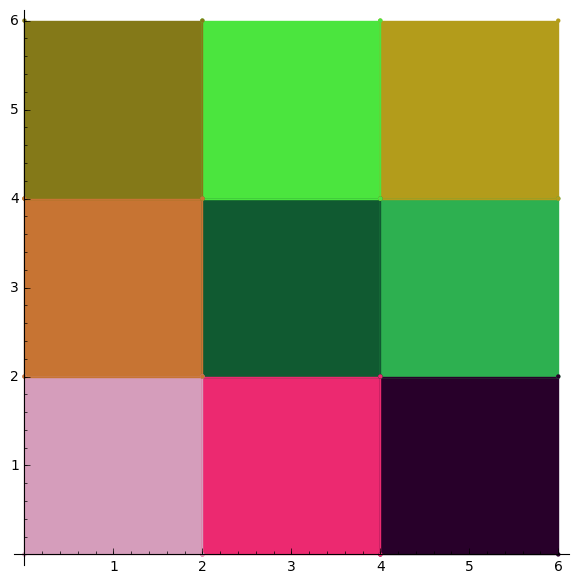
Region of evaluation, \(R\).
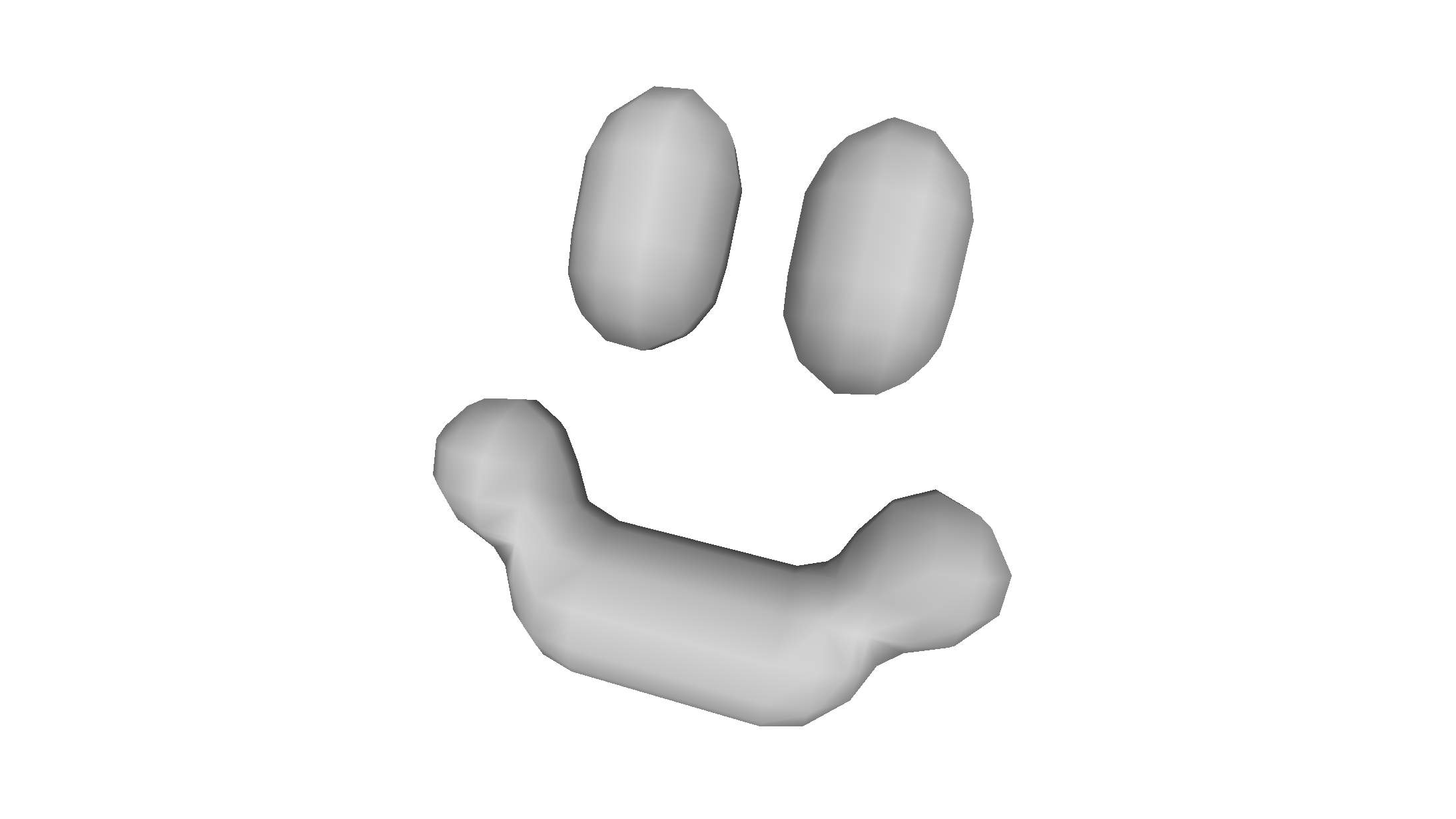
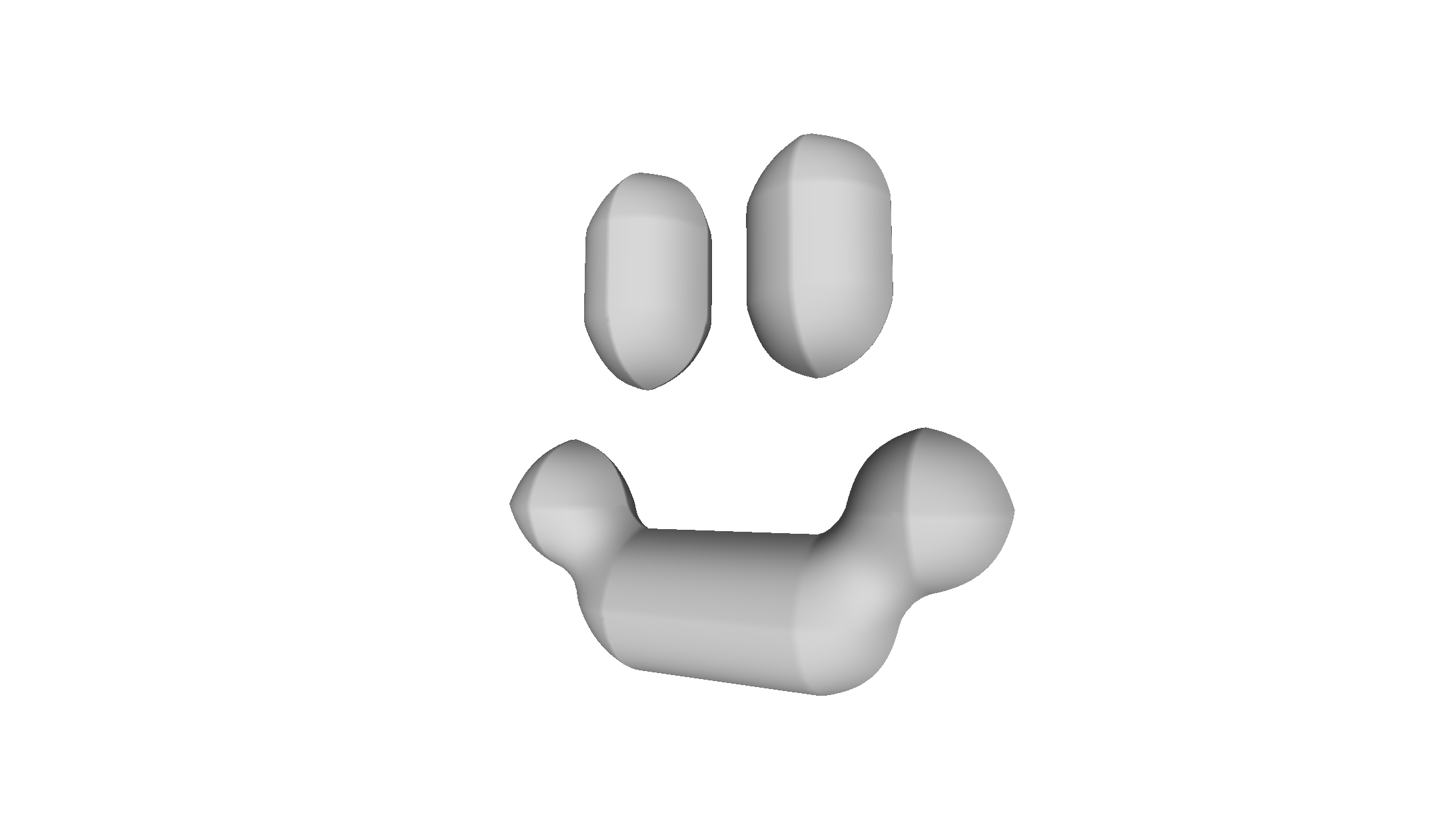
\(\rho(x)\) is this shift
Fast Evaluation
Sub-regions
\(S_1\)
\(S_2\)
\(S_3\)
\(S_4\)
Fast Evaluation
So assume \(x\in R\). For each sub-region \(j\) we define \(\psi_j\) with
\displaystyle\sum_{n\in C_0(x)} c_n \ \varphi\left(x-n\right)
For box splines, we distribute the polynomial pieces into their corresponding sub-regions, i.e. \(\psi_i\). we can then spend time simplifying the polynomial \(\psi_i\)
= \Psi(x)
\Psi(x) := \begin{cases}
\psi_1(x) & x \in S_1 \\
\ & \vdots\\
\psi_M(x) & x \in S_M
\end{cases}
so that
Fast Evaluation
\(c_{0,0}\)
\(c_{1,0}\)
\(c_{1,1}\)
\(c_{0,1}\)
\(c_{-1,1}\)
\(c_{-1,0}\)
\(c_{-1,-1}\)
\(c_{0,-1}\)
\(c_{2,-1}\)
Fast Evaluation
\(c_{0,0}\)
\(c_{1,0}\)
\(c_{1,1}\)
\(c_{0,1}\)
\(c_{-1,1}\)
\(c_{-1,0}\)
\(c_{-1,-1}\)
\(c_{0,-1}\)
\(c_{2,-1}\)
\(C_0(R_1)\)
Fast Evaluation
\(c_{0,0}\)
\(c_{1,0}\)
\(c_{1,1}\)
\(c_{0,1}\)
\(c_{-1,1}\)
\(c_{-1,0}\)
\(c_{-1,-1}\)
\(c_{0,-1}\)
\(c_{2,-1}\)
\(C_0(R_2)\)
Fast Evaluation
\(c_{0,0}\)
\(c_{1,0}\)
\(c_{1,1}\)
\(c_{0,1}\)
\(c_{-1,1}\)
\(c_{-1,0}\)
\(c_{-1,-1}\)
\(c_{0,-1}\)
\(c_{2,-1}\)
\(C_0(R_3)\)
Fast Evaluation
\(c_{0,0}\)
\(c_{1,0}\)
\(c_{1,1}\)
\(c_{0,1}\)
\(c_{-1,1}\)
\(c_{-1,0}\)
\(c_{-1,-1}\)
\(c_{0,-1}\)
\(c_{2,-1}\)
\(C_0(R_4)\)
Fast Evaluation
Assume \(x\in R\). For fix some \(j\) we define \(\psi_j\) with
\psi_j(x) = \displaystyle\sum_{n\in C_0(S_j)} c_n \ \varphi\left(x-n\right)
We know that \(\varphi\) is a polynomial for all points \(x\in S_j\), so we can write it as
\psi_j(x) = \displaystyle\sum_{n\in C_0(S_j)} c_n \ P_n(x)
For some polynomial \(P_n(x)\)
Fast Evaluation
For the last example
\psi_1(x) = \displaystyle\sum_{n\in C_0(S_1)} c_n \ \varphi\left(x-n\right)
$$\psi_1=c_{-1,1}\varphi\left(x-(-1,1)\right) + c_{1,1} \varphi\left(x-(-1,1)\right)$$ $$ + c_{-1,0} \varphi\left(x-(-1,0)\right) + c_{1,0} \varphi\left(x-(1,0)\right) $$ $$ + c_{0,1} \varphi\left(x-(0,1)\right) + c_{0,0} \varphi\left(x-(0,0)\right)$$ $$ +c_{0,-1} \varphi\left(x-(0,-1)\right)$$
$$1/4(c_{-1,-1} + c_{-1,0} - 2c_{0,-1} - 2c_{0,0} + c_{1,-1} + c_{1,0})x_0^2 $$ $$+ 1/4(c_{-1,-1} - c_{-1,0} - 2c_{0,0} + 2c_{0,1} + c_{1,-1} - c_{1,0})x_1^2 $$ $$- 1/2(c_{-1,0} - c_{1,0})x_0 $$ $$+ 1/2((c_{-1,-1} - c_{-1,0} - c_{1,-1} + c_{1,0})x_0 - c_{0,-1} + c_{0,1})x_1 + 1/8c_{-1,0} $$ $$ + 1/8c_{0,-1} + 1/2c_{0,0} + 1/8c_{0,1} + 1/8c_{1,0})$$
$$\psi_1=$$
Fast Evaluation
We can explicitly calculate each region
$$\psi_3(x)=1/4(c_{-1,-1} + c_{-1,0} - 2c_{0,-1} - 2c_{0,0} + c_{1,-1} + c_{1,0})x_0^2 + 1/4(c_{-1,-1} - c_{-1,0} - 2c_{0,0} + 2c_{0,1} $$ $$+ c_{1,-1} - c_{1,0})x_1^2 - 1/2(c_{-1,0} - c_{1,0})x_0 + 1/2((c_{-1,-1} - c_{-1,0} - c_{1,-1} + c_{1,0})x_0 - c_{0,-1} + c_{0,1})x_1 $$ $$+ 1/8c_{-1,0}+ 1/8c_{0,-1} + 1/2c_{0,0} + 1/8c_{0,1} + 1/8c_{1,0}'$$
$$\psi_2(x)=1/4(2c_{-1,0} - c_{0,-1} - 2c_{0,0} - c_{0,1} + c_{1,-1} + c_{1,1})x_0^2 + 1/4(c_{0,-1} - 2c_{0,0} + c_{0,1} + c_{1,-1}$$ $$ - 2c_{1,0} + c_{1,1})x_1^2 - 1/2(c_{-1,0} - c_{1,0})x_0 + 1/2((c_{0,-1} - c_{0,1} - c_{1,-1} + c_{1,1})x_0 - c_{0,-1} + c_{0,1})x_1$$ $$ + 1/8c_{-1,0}+ 1/8c_{0,-1} + 1/2c_{0,0} + 1/8c_{0,1} + 1/8c_{1,0}$$
$$\psi_1(x)=1/4(c_{-1,0} + c_{-1,1} - 2c_{0,0} - 2c_{0,1} + c_{1,0} + c_{1,1})x_0^2 - 1/4(c_{-1,0} - c_{-1,1} - 2c_{0,-1} $$ $$+ 2c_{0,0} + c_{1,0} - c_{1,1})x_1^2 - 1/2(c_{-1,0} - c_{1,0})x_0 + 1/2((c_{-1,0} - c_{-1,1} - c_{1,0} + c_{1,1})x_0 $$ $$- c_{0,-1} + c_{0,1})x_1 + 1/8c_{-1,0} + 1/8c_{0,-1} + 1/2c_{0,0} + 1/8c_{0,1} + 1/8c_{1,0}$$
$$\psi_4(x)=1/4(c_{-1,-1} + c_{-1,1} - c_{0,-1} - 2c_{0,0} - c_{0,1} + 2c_{1,0})x_0^2 + 1/4(c_{-1,-1} - 2c_{-1,0} + c_{-1,1} + c_{0,-1} $$ $$- 2c_{0,0} + c_{0,1})x_1^2 - 1/2(c_{-1,0} - c_{1,0})x_0 + 1/2((c_{-1,-1} - c_{-1,1} - c_{0,-1} + c_{0,1})x_0 - c_{0,-1} + c_{0,1})x_1 $$ $$+ 1/8c_{-1,0} + 1/8c_{0,-1} + 1/2c_{0,0} + 1/8c_{0,1} + 1/8c_{1,0}$$
Fast Evaluation
Now what? We have a list of polynomials but there are still branches necessary, i.e.
\Psi(x) := \begin{cases}
\psi_1(x) & x \in S_1 \\
\ & \vdots\\
\psi_M(x) & x \in S_M
\end{cases}
This great on modern CPU architectures, but is not so good on GPU architectures. Multiple cases = branches.
If we fail, we'll drop back to branch predication
We could try branch predication, but this is quite wasteful. Let's try to be more clever.
Fast Evaluation
For the last example
$$=1/4(k_1 + k_2 - 2k_4 - 2k_5 + k_7 + k_8)x_0^2 $$ $$- 1/4(k_1 - k_2 - 2k_3 + 2k_4 + k_7 - k_8)x_1^2 $$ $$- 1/2(k_1 - k_7)x_0 + 1/2((k_1 - k_2 - k_7 + k_8)x_0 - k_3 + k_5)x_1$$ $$ + 1/8k_1 + 1/8k_3 + 1/2k_4 + 1/8k_5 + 1/8k_7$$
\(\psi^*(x_0,x_1, k_1, k_2, k_3, k_4,k_5,k_6,k_7)\)
Then
\psi_1(x) = \psi^*(x_0 , x_1 , c_{-1, 0}, c_{0, -1}, c_{0, 0}, c_{0, 1}, c_{1, -1}, c_{1, 0}, c_{1, 1})
\psi_2(x) = \psi^*(x_1 , x_0 , c_{0, -1}, c_{1, -1}, c_{-1, 0}, c_{0, 0}, c_{1, 0}, c_{0, 1}, c_{1, 1})
\psi_3(x) = \psi^*(-x_0 , -x_1 , c_{1, 1}, c_{1, 0}, c_{1, -1}, c_{0, 1}, c_{0, 0}, c_{0, -1}, c_{-1, 0})
\psi_4(x) = \psi^*(-x_1 , -x_0 , c_{1, 1}, c_{0, 1}, c_{1, 0}, c_{0, 0}, c_{-1, 0}, c_{1, -1}, c_{0, -1})
We only need to know one polynomial!
Fast Evaluation
There is no guarantee that we'll only have one \(\psi^*\), so we may have a set of such functions. We want to find a minimal set of \(\{\psi^*_j\}\), that contains the set \(\{\psi_1 \cdots \psi_M\}\) under rotations and translations of the elements of \(\{\psi_j^*\}\)
Rotations and translations can be stored in a lookup table for GPU evaluation.
Minimize the amount of elements \(\{\psi_j^*\}\) has, since having multiple leads to either branching or additional wasted work on the GPU
Fast Evaluation
How do we evaluate the polynomials?
Recall Horner's method
f(x) = \displaystyle\sum^n_{k=1} a_k x^k = a_0 + a_1x + \cdots + a_{n-1}x^{n-1} + a_nx^n
f(x) = \displaystyle\sum^n_{k=1} a_k x^k = a_0 x(a_1 + ... + x(a_{n-1} + a_nx))
There is no such unique factorization with more than one variable
Fast Evaluation
That's fine, Horner factorization still exist, let's just brute force search for them
f({x}) = c_1x_1x_2x_3x_4 + c_2x_2x_3x_4x_5 + c_3x_1x_3x_4x_5 + c_4x_1x_2x_4x_5 + c_5x_1x_2x_3x_5 + c_6
f({x}) = x_3x_4(x_2(c_1x_1+c_2x_5) + c_3x_1x_5) + x_1x_2x_5(c_4x_4 + c_5x_3) + c_6
12 muliplications
Fast Evaluation
Efficiently compute the monomials
We get these for free on the GPU, these can be evaluated while waiting for texture reads
x_1
x_2
x_3
x_4
x_5
x_1x_2
x_1x_5
x_3x_4
x_1x_2x_5
4 multiplications - leaves 8 in previous form
Fast Evaluation
General outline
f = 0
for each coset j:
    n = rho(x) // Linear transform
    x = x - n

    sub_reg_idx = planeLookup(x)
    C = coeffPermutationLookup[sub_reg_idx]
    R = localTransformLookup[sub_reg_idx]
    t = localTranslateLookup[sub_reg_idx]

    coeffs = accessCoefficients(sub_reg_idx, n)

    f += Psi(j, R*x + t, coeffs); // use effecient monom eval
return f;
Fast Evaluation
static __forceinline__ __device__ float convolution_sum(const body_centered_cubic *l, const float &u, const float &v, const float &w,
unsigned char *region_lut_s,
unsigned char *ls_lut_s,
unsigned char *sr_lut_s,
char *sites_s,
unsigned char *vperm_s,
float* shared_bank) {
float x_0, x_1, x_2;
int vx, vy, vz;
int thread_id = (threadIdx.y * blockDim.x) + threadIdx.x;
float *s = &shared_bank[thread_id*4];
// Lookups...
return 0.5*((-r3 + r4)*v_0 +
(r1 - r2)*v_1 +
(r1 + r2 - r3 - r4)*v_2 +
(2.)*r3);
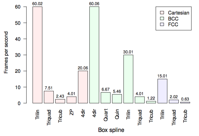
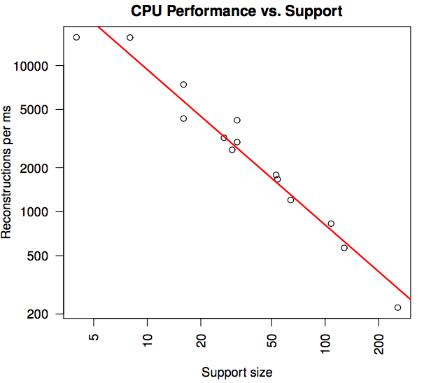
}Experiments
CPU Performance, GPU Performance, Volumetric Rendering
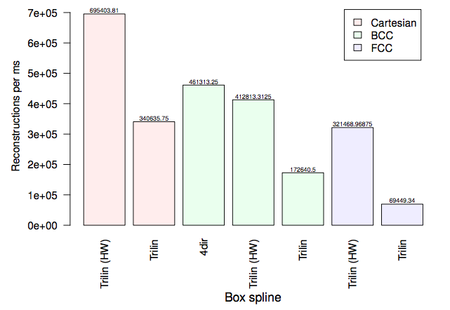
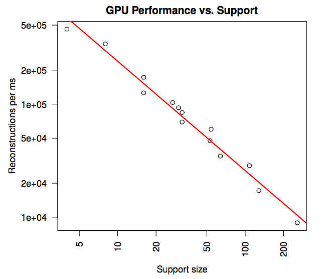
Results
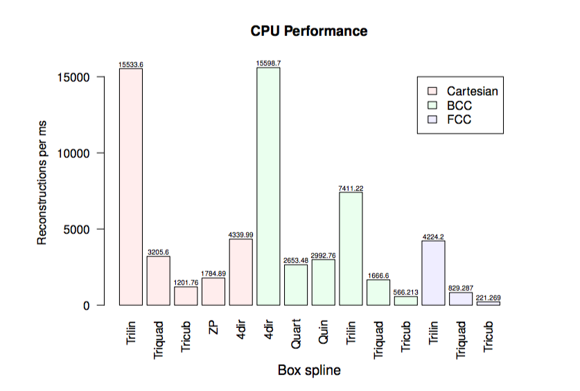
Results
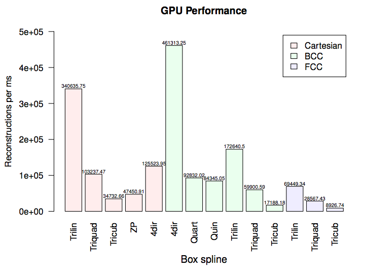
No hardware acceleration*
Experiments
Results
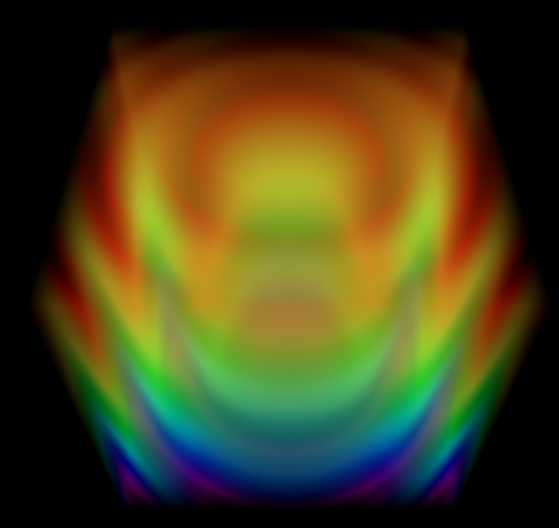
Volume Rendering
Results
Results
Conclusion
This allows us to build a general interpolation library, on regular grids, that is well suited to experimentation and speed
Lots of stuff I haven't talked about
- Filtering
- Fourier Transforms
- Compression
Fast Splines
By Joshua Horacsek


