Double-Bracket Algorithmic Cooling
(DBAC)
Kay Giang - NTU Singapore
Ingredients for DBAC
- Quantum Dynamic Programming
- Algorithmic Cooling
- Quantum Imaginary Time Evolution
First ingredient:
Quantum Dynamic Programming (QDP)

- Usual quantum computing is static: To change operation \(\to\) have to change the circuit
- Dynamic quantum computing: To change operation, only need to change instruction qubit
Normal way we do quantum computing: Static
Dynamic Quantum Computing
Kjaergaard et al., arxiv:2001.08838
Unfolding quantum recurions
Consider Grover reflector: \(G=id - 2\ket\psi\bra\psi\)
\(Q,R \in U(D)\), initial state \(\ket{\psi_0}\), \(\ket{\psi_{k+1}} = QG^{(\psi_k)}R\ket{\psi_k}\)
\begin{align*}
G^{(\psi_1)}
&=\mathbb{1} - 2\ket{\psi_1}\bra{\psi_1}\\
&=\mathbb{1} - 2U(\psi_0) \ket{\psi_0}\bra{\psi_0}U(\psi_0)^\dagger\\
&=U(\psi_0)(\mathbb{1}-2\ket{\psi_0}\bra{\psi_0})U(\psi_0)^\dagger\\
&= U(\psi_0) G^{(\psi_0)}U(\psi_0)^\dagger
\end{align*}
\begin{align*}
U(\psi_0) &= QG^{(\psi_0)}R\\
\ket{\psi_1} &= QG^{(\psi_0)}R\ket{\psi_0}
\end{align*}
However, it's more complicated to get \(\ket{\psi_2}\). To do this, we need to get \(U(\psi_1)\). Ordinary idea:
Reflection of \(\psi_1\) is the rotated reflection of \(\psi_0\)
To get \(\ket{\psi_1}\) is simple:
\begin{align*}
\ket{\psi_2} &= QG^{(\psi_1)}R\ket{\psi_1}\\
&={Q(QG^{(\psi_0)}R)G^{(\psi_0)}(QG^{(\psi_0)}R)^\dagger R QG^{(\psi_0)}R\ket{\psi_0}}
\end{align*}
Why use QDP?
- Unfolding the recursion make the depth grow exponentially
- Using placeholder memory is not straightforward with quantum computing
- Quantum Dynamic Programming (QDP), a framework that uses copies of the recursive state to implement the recursion step unitary
Why use QDP?
- QDP yields exponential reduction in circuit depth than when unfolding
- QDP is dynamic because the instruction state is revealed only on runtime
- Kimmel et al. (arxiv 1608.00281) shows that using quantum information as source code is basis of a universal model for quantum computation
Quantum Dynamic Programming
- QDP speed up recursion of the form (single memory call):
\[ U^{(\mathcal{N},\rho)} = V_2e^{i\mathcal{N}(\rho)}V_1\] where \(\mathcal{N}\) is any Hermitian-preserving map - Memory call: Idealized transformation we want to make. It asks for memory (instruction state \(\rho\)).
- General case:
- Problem: We can't implement this naturally in qunatum mechanics

Quantum Dynamic Programming
- Solution: QDP approximate this memory call unitary:
- QDP does this by using memory usage query:
where \(N\) is the operator of the memory usage query, the partial transpose of the Choi matrix corresponding to \(\mathcal{N}\)- Consume (trace out) an instruction state
- Repeat this procedure M times, we obtain
\mathcal{E}_s^{(N,\rho)}(\sigma) = Tr_\rho [e^{-iNs} (\rho\otimes\sigma) e^{iNs}]
E^{(\mathcal{N},\rho)}(\sigma) = e^{i\mathcal{N}(\rho)} \sigma e^{-i\mathcal{N}(\rho)}
\mathcal{E}^{(\mathcal{N},\rho,M)}_{QDP} \coloneqq (\mathcal{E}^{(\mathcal{N},\rho)}_{1/M})^M = E^{(\mathcal{N},\rho)} + O(1/M)
Second ingrdient:
Algorithmic Cooling (AC)
- Set-up: \(n\) qubits identically prepared
- Objective: minimize 1 particular qubit entropy
- Method: apply a global unitary operation iteratively
- AC acts on mixed state with initial polarisation
\[\rho = \begin{pmatrix}p & 0 \\0 & 1 - p\end{pmatrix}\] - AC works by redistributing \(|0\rangle\) and \(|1\rangle\) population
Extreme case: Pure state
Question: What if the state is pure (but not in computational basis)?
\(\to\) AC suppress coherence at expense of adding entropy
\(\to\) Cooling to a pure ground state is then not possible
Single qubit rotation can rotate a pure qubit to perfect ground state \(|\psi\rangle\to|0\rangle\)
\(\to\) Can we handle coherence via single qubit rotation?
\(\to\) Yes, with double-bracket algorithmic cooling
Third ingredient:
Quantum imaginary time evolution (QITE)
|\Psi(\tau)\rangle = \frac{e^{-\tau \hat{H}}}{\|e^{-\tau \hat{H}}|\Psi(0)\rangle\|} |\Psi(0)\rangle
\(\Psi(0)\): Initial state
\(\Psi(\tau)\): State at time \(\tau\)
\(\hat H\): Diagonalised Hamiltonian
Cool the initial state \(\Psi(0)\) with respect to the Hamiltonian \(\hat H\)
DB-QITE formula
|\Psi(\tau)\rangle = \frac{e^{-\tau \hat{H}}}{\|e^{-\tau \hat{H}}|\Psi(0)\rangle\|} |\Psi(0)\rangle
Gluza et al. (2412.04554) shows that QITE satisfy:
\begin{align*}
\partial_\tau {|\Psi(\tau) \rangle} = [\Psi(\tau),\hat{H}] |\Psi(\tau) \rangle
\end{align*}
Double-bracket
\frac{\partial \Psi(\tau)}{\partial \tau} = \big[ [\Psi(\tau),\hat H],\Psi(\tau)\big]
In terms of the density matrix \(\Psi(\tau)\):
Recursion step
\ket{\Psi(t)}\approx e^{t[\Psi(0),\hat H]}\ket{\Psi_0}
For short duration t:
\partial_\tau {|\Psi(\tau) \rangle} = [\Psi(\tau),\hat{H}] |\Psi(\tau) \rangle\
This motivates defining the recursion step:
\ket{\psi_{k+1}} = e^{t_k[\psi_k,\hat H]} \ket{\psi_k}
\(\ket{\psi_k}\): State at step \(k\)
DB-QITE recursion formula
\boxed{\ket{\psi_{k+1}} \approx e^{i\sqrt{t_k}\hat H} e^{i\sqrt{t_k}\psi_k}
e^{-i\sqrt{t_k}\hat H}\ket{\psi_k}}
e^{t[\psi,\hat H]}|\psi\rangle =
e^{i\sqrt{t}\hat H}e^{i\sqrt{t}\psi}
e^{-i\sqrt{t}\hat H}
e^{-i\sqrt{t}\psi}|\psi\rangle + \mathcal O(t^{3/2})
Using the group commutator relation:
DB-QITE recursion formula:
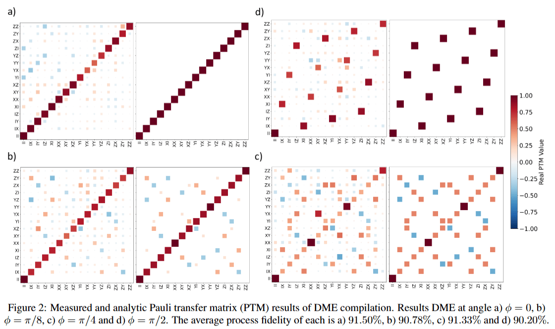
Density matrix exponentiation (DME)
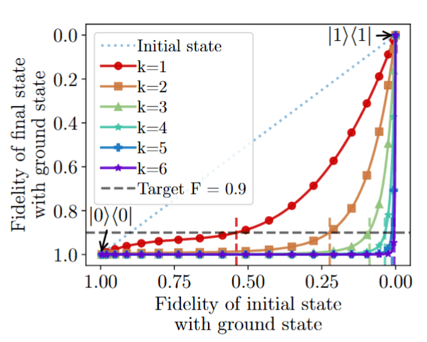
DB-QITE Performance
\boxed{\ket{\psi_{k+1}} \approx e^{i\sqrt{t_k}\hat H} e^{i\sqrt{t_k}\psi_k}
e^{-i\sqrt{t_k}\hat H}\ket{\psi_k}}
If we have ideal DME
\(e^{i\sqrt{t_k}\psi_k}\)
Ingredients for DBAC
- Quantum Dynamic Programming (QDP)
- Algorithmic Cooling (AC)
- Quantum Imaginary Time Evolution (QITE)
Double-bracket Algorithmic Cooling (DBAC)
Set up of DBAC protocol
- Set-up: \(n\) qubits identically prepared in a pure state \(|\psi\rangle\)
- Objective: rotate 1 qubit to ground state \(|0\rangle\)
- Method: Simulating imaginary time evolution by compiling a circuit
Compilation for resetting one qubit
\boxed{\ket{\psi_{k+1}} \approx e^{i\sqrt{t_k}\hat H} e^{i\sqrt{t_k}\psi_k}
e^{-i\sqrt{t_k}\hat H}\ket{\psi_k}}
\(e^{i\sqrt{t_k}\psi_k}\): Density matrix exponentiation (DME)
Single qubit: \(\hat H = \hat Z\)
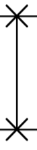
: \(\delta\)SWAP gate, applying \(e^{-i t \text{SWAP}}\). Compiled using Heisenberg interaction: \(e^{it(XX+YY+ZZ)}\)
DME Circuit
\boxed{\ket{\psi_{k+1}} \approx e^{i\sqrt{t_k}\hat H} e^{i\sqrt{t_k}\psi_k}
e^{-i\sqrt{t_k}\hat H}\ket{\psi_k}}
DME Circuit
\(\delta\)SWAP compiled using Heisenberg interaction: \(e^{it(XX+YY+ZZ)}\)

DME Circuit
Reason for using ZZ interaction: The entangling operation in transmon qubit is Stark-induced ZZ by level excursions (siZZle)
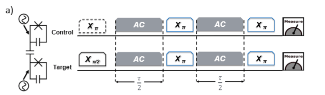
DME experimental calibration
Energy reduction guarantee
E_\text{DBAC} = E_0-2\sin^2(t)(1-E_0^2)\Big((1-\cos(t)) E_0 - \cos(t)\Big)
Energy after 1 step:
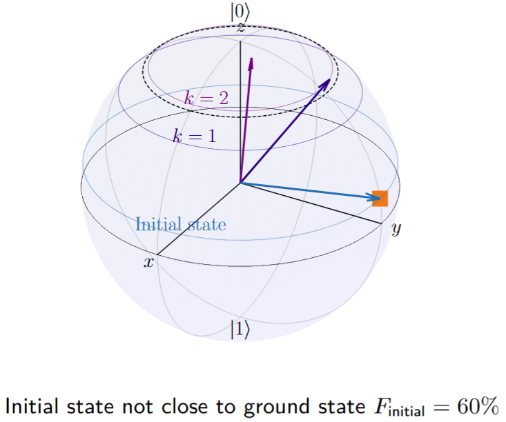
Rotation on Bloch sphere
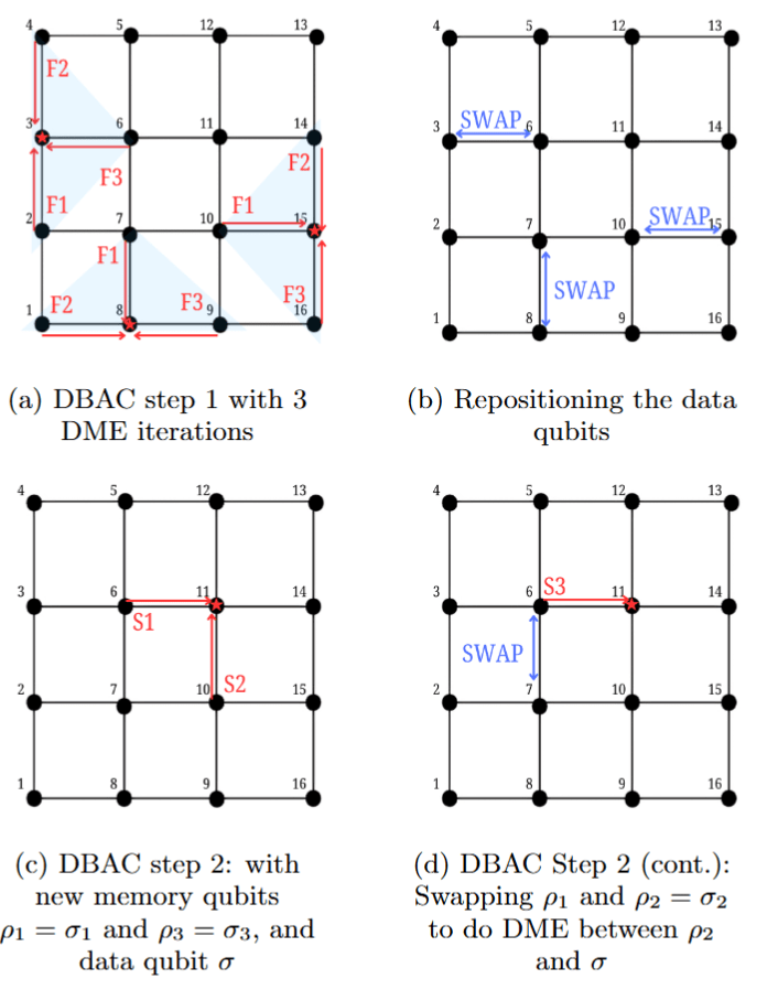
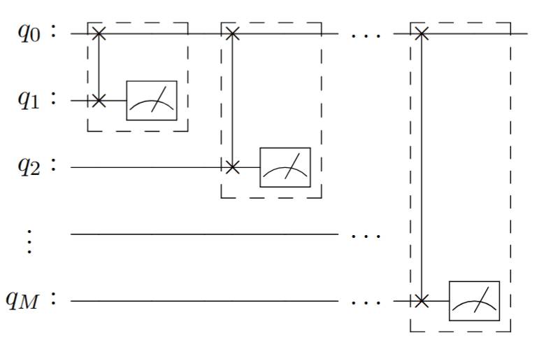
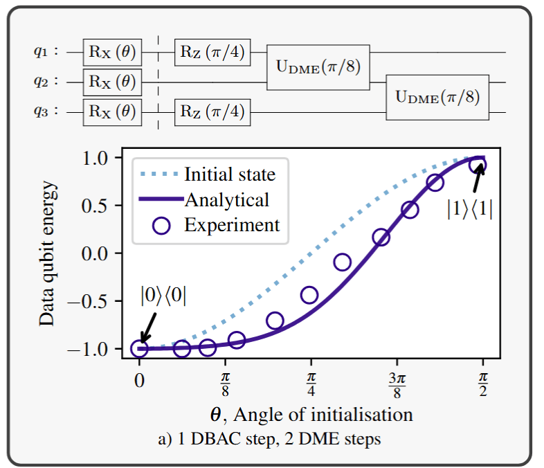
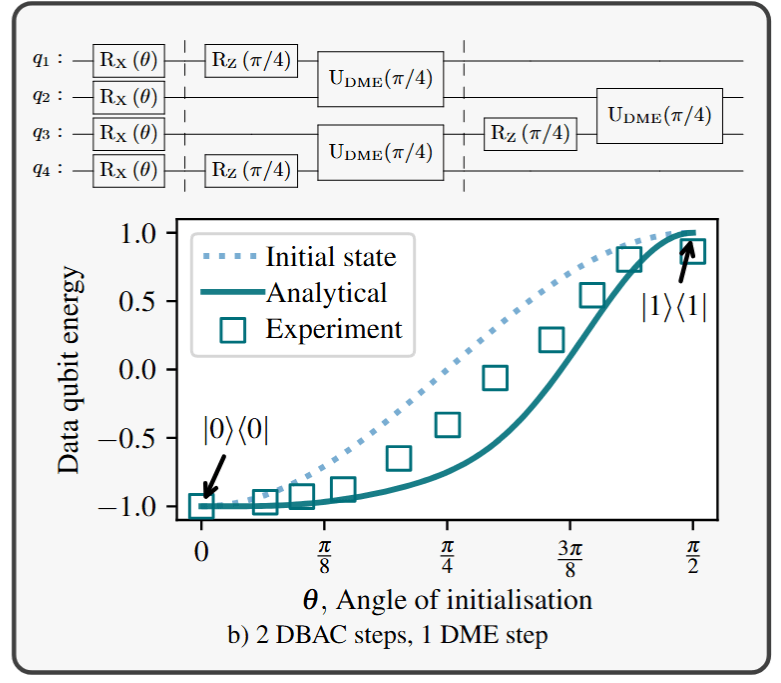
Example layout for 2 steps of DBAC with 3 DME iterations in each
Why use DBAC?
- Naive method for resetting qubit via rotation: tomography
- Central limit theorem: Statistical error e.g. \(\langle X\rangle\) estimation scale as \(1/\sqrt{n}\)
- DBAC uses less copies, because it is dynamic so we don't need to know the state precisely
- DBAC is the first protocol experimentally tested, where the dynamic aspect has a clear physics utility
- This is our first step towards building a quantum dynamic tool-kit
Summary
- DBAC setting: \(n\) qubits initialised to the same pure state \(|\psi\rangle\)
- DBAC simulates imaginary time evolution via a hardware native compilation to cool the coherence of one qubit to ground state \(|0\rangle\)
- DBAC is part of a dynamic quantum tool-kit that offers exponential circuit depth reduction
Thank you for listening!
DBAC
By Khanh Uyen Giang


