Ensemble Data Assimilation in
High-Dimensional Chaotic Systems:
Exploiting Low-Dimensional Structures
Kota Takeda
Nagoya University, Japan
* The author was supported by RIKEN Junior Research Associate Program and JST SPRING JPMJSP2110.
\Psi
\Psi
Self-introduction
Kota Takeda

Assistant Prof.
at Nagoya Univ., Japan
Research topics:
Uncertainty Quantification
Fluid mechanics
Data assimilation
Nagoya

SIAM activities
(Past) President
of SIAM Student Chapter Kyoto
Joining
SIAM-related Conference held
at Japan, Macau, HongKong, U.S., Italy, & Korea
Establishing publications
in SIAM/JSIAM Journals
This slide is shared.
and so on...

Visit my website!
Contents
-
Introduction
- Numerical Weather Prediction
-
Background
- Mathematical formulation, Ensemble Kalman filter
-
Recent Studies
- Literature, Exploiting low-dimensionality, Conjecture
-
Numerical Result
- Result supporting the conjecture
- Summary
Numerical Weather Prediction
Introduction
Numerical Weather Prediction
Numerical Weather Prediction
State estimation of High dimensional chaotic system

Numerical Weather Prediction
Numerical Weather Prediction
State estimation of High dimensional chaotic system
Unpredictable in long-term

e.g., Typhoon forecast circles
\sim 10^8
3D grid × variable
Numerical Weather Prediction
Numerical Weather Prediction
State estimation of High dimensional chaotic system

\sim 10^8
3D grid × variable
We only have partial and noisy observations
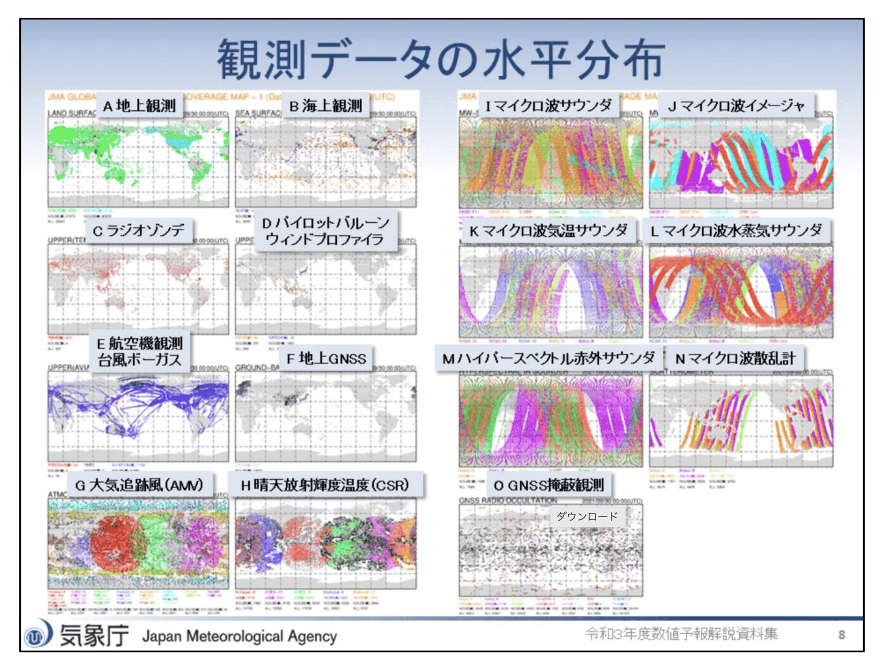
気象庁
Numerical Weather Prediction
Numerical Weather Prediction
State estimation of High dimensional chaotic system
気象庁
(x,y,z)\mapsto(x,y)
noise
partial
idealize
chaotic
\sim 10^8
3D grid × variable
We only have partial and noisy observations
Numerical Weather Prediction
Numerical Weather Prediction
State estimation of High dimensional chaotic system
We only have partial and noisy observations
気象庁
(x,y,z)\\
\mapsto(x,y)
noise
partial
chaotic
idealize
\sim 10^8
3D grid × variable
Mathematical formulations
(x,y,z)\\
\mapsto(x,y)
noise
partial
chaotic
Background
Mathematical formulations

\mathbb{R}^{N_x}
The known model generates an unknown true trajectory.
t
unknown trajectory
\frac{d u}{dt} = \mathcal{F}(u)
(\mathcal{F}: \mathbb{R}^{N_x} \rightarrow \mathbb{R}^{N_x}, u(0) = u_0 \in \mathbb{R}^{N_x})
u(t) = \Psi_t (u_0)
Model dynamics
Semi-group
solution
(\Psi_t : \mathbb{R}^{N_x} \rightarrow \mathbb{R}^{N_x}, t \ge 0)
(assume)
unknown
known
(x,y,z)\\
\mapsto(x,y)
noise
partial
chaotic
unknown
Mathematical formulations
u_{n} = \Psi (u_{n-1})
(\Psi = \Psi_\tau)
known
\mathbb{R}^{N_x}
t
unknown trajectory
u_1
u_2
t_1
t_2
t_3
...
\tau
\Psi
y_n = H u_n + \eta_n
(H \in \mathbb{R}^{N_y}, \eta_n \sim \mathcal{N}(0, R))
Gaussian
y_1
y_2
\in \mathbb{R}^{N_y}
\in \mathbb{R}^{N_y}
\mathbb{R}^{N_y}
at discrete time steps.
\tau
\tau > 0:
observation interval
We have noisy observations in
Observation
Discrete-time model
(x,y,z)\\
\mapsto(x,y)
noise
partial
chaotic
u_{n}
y_n
Mathematical formulations
\mathbb{R}^{N_x}
t
t_1
t_2
t_3
\tau
\tau
(x,y,z)\\
\mapsto(x,y)
noise
partial
chaotic
y_1
y_2
...
y_2
y_3
u_1
u_2
u_3
\Psi
\Psi
Sequential state estimation
using the 'background' information
given
y_{1:n} = \{y_i \mid i \le n\}
Filtering problem
u_n
estimate
\text{For } n \in \mathbb{N},
known:
\Psi,
H,
obs. noise distribution.
u_{n}
y_n
Mathematical formulations
\mathbb{R}^{N_x}
t
t_1
t_2
t_3
\tau
\tau
y_1
y_2
...
y_2
y_3
u_1
u_2
u_3
\Psi
\Psi
given
y_{1:n} = \{y_i \mid i \le n\}
Filtering problem
u_n
estimate
known:
'background info.'
Bayesian data assimilation
approximate
\mathbb{P}^{u_n}({}\cdot{}| \qquad )
(conditional distribution)
y_{1:n}

\mathbb{P}^{u_2}({}\cdot{}|y_{1:2} )
\mathbb{P}^{u_1}({}\cdot{}|y_1 )
\mathbb{P}^{u_3}({}\cdot{}|y_{1:3} )
Mathematical formulations
\mathbb{R}^{N_x}
t
t_1
t_2
t_3
\tau
\tau
y_1
y_2
y_2
y_3
\mathbb{P}^{v_{n-1}}
\mathbb{P}^{u_n}({}\cdot{}| y_{1:n} ) \approx \mathbb{P}^{v_n}
Bayesian data assimilation
approximate
v_n
※ Estimates of
y_{1:n}
using
a recursive update of
\mathbb{P}^{v_n}
u_1
u_2
u_3
u_n
for efficiency!
Construct
Mathematical formulations
\mathbb{R}^{N_x}
t
t_1
t_2
t_3
\tau
\tau
y_1
y_2
y_2
y_3
\mathbb{P}^{v_{n-1}}

(I) Prediction
\Psi
\mathbb{P}^{\hat{v}_n}
(I) Prediction
by model
\mathbb{P}^{u_n}({}\cdot{}| y_{1:n} ) \approx \mathbb{P}^{v_n}
Bayesian data assimilation
approximate
v_n
\hat{v}_n
※ Estimates of
y_{1:n}
y_{1:n-1}
using
using
recursive update of
\mathbb{P}^{v_n}
u_1
u_2
u_3
u_n
Introducing auxiliary var.,
'prediction'!
Mathematical formulations
\mathbb{R}^{N_x}
t
t_1
t_2
t_3
\tau
\tau
y_1
y_2
y_2
y_3
\mathbb{P}^{v_{n-1}}
y_n
(II)Analysis
(II) Analysis
\mathbb{P}^{v_n}
by Bayes' rule
\mathbb{P}^{v_n} \propto L_{y_n} \cdot \mathbb{P}^{\hat{v}_n}
likelihood function
(I) Prediction
\Psi
\mathbb{P}^{\hat{v}_n}
(I) Prediction
by model
\mathbb{P}^{u_n}({}\cdot{}| y_{1:n} ) \approx \mathbb{P}^{v_n}
Bayesian data assimilation
approximate
v_n
\hat{v}_n
※ Estimates of
y_{1:n}
y_{1:n-1}
using
using
recursive update of
\mathbb{P}^{v_n}
u_1
u_2
u_3
u_n
Repeat (I) & (II)
Prediction
...
\Rightarrow \mathbb{P}^{v_n} = \mathbb{P}^{u_n}({}\cdot{} | \bm{y}_n).
Proposition
\text{Assume } \mathbb{P}^{v_0} = \mathbb{P}^{u_0}.
The n-iterations (I) & (II)
A major ensemble data assimilation algorithm
Background
Ensemble Kalman filter (EnKF)
'Ensemble' → Approximate by a set of particles
'Kalman' → Gaussian approximation
→ Correct mean and covariance
using observation
ensemble
a set of particles (samples)!
V_n = (v_n^{(k)})_{k=1}^m
\mathbb{P}^{v_n}
A major ensemble data assimilation algorithm
Ensemble Kalman filter (EnKF)
(Evensen2009)
- Approximate by ensemble
- Update:
- Correct mean and covariance
using observation
\mathbb{R}^{N_x}
t
y_1
y_2
t_1
t_2
t_3
\tau
t_0
Repeat (I) & (II)...
(II)Analysis
(I) Prediction
\Psi
v_0^{(1)}
v_0^{(m)}
v_0^{(2)}


\widehat{v}_1^{(1)}
v_1^{(1)}
\vdots
\widehat{v}_1^{(m)}
v_1^{(m)}
Just evolve each sample
Correct samples based on the least squares
V_{n-1} \overset{(I)}{\rightarrow} \widehat{V}_n \overset{(II)}{\rightarrow} V_n
Ensemble Kalman filter (EnKF)
V_n = (v_n^{(k)})_{k=1}^m, \widehat{V}_n = (\widehat{v}_n^{(k)})_{k=1}^m
ensemble
(Evensen2009)
m
ensemble size
Ensemble Kalman filter (EnKF)
Question
How many samples are required
for 'accurate state estimation' using EnKF?
m
ensemble size
\limsup_{n\rightarrow \infty}\mathbb{E}[|\delta_n|^2] = O(r^2),
(Asymptotic) filter accuracy
\delta_n = u_n - \overline{v}_n
: state estimation error.
r^2
: variance of obs. noise,
where
\overline{v}_n = \textstyle{\frac{1}{m} \sum_{k=1}^m v^{(k)}_n}
estimate of EnKF
r
squared error
log-log
O(r^2)
Ensemble Kalman filter (EnKF)
Question
How many samples are required
for 'accurate state estimation' using EnKF?
m
ensemble size
ensemble
Large
m
Accurate
m
Small
m
ensemble
Inaccurate
← Find minimum
achieving accuracy!
m = m^*
r
squared error
log-log
O(r^2)
Ensemble Kalman filter (EnKF)
Question
How many samples are required
for 'accurate state estimation' using EnKF?
Recent Studies
Literature
(de Wiljes+2018, T.+2024)
(Sanz-Alonso+2025)
(González-Tokman+2013)
m \ge N_x + 1
m \ge 6 N_y
m \ge N_+ + 1
for
using
'Stability' of
\Psi
in unobserved sp.
\Psi
'Lipschitz'
with
too many
additional factor
Accurate initial ensemble
unrealistic
Mathematical analyses have revealed sufficient conditions for .
m
N_+:
Dim. of 'unstable directions'
in tangent sp.
Literature
(de Wiljes+2018, T.+2024)
(Sanz-Alonso+2025)
(González-Tokman+2013)
m \ge N_x + 1
m \ge 6 N_y
m \ge N_+ + 1
for
using
'Stability' of
\Psi
in unobserved sp.
\Psi
'Lipschitz'
with
N_+:
Dim. of 'unstable directions'
in tangent sp.
too many
additional factor
Accurate initial ensemble
unrealistic
Mathematical analyses have revealed sufficient conditions for .
m
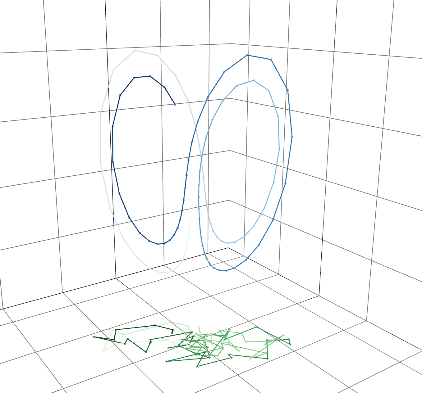
Focus on
Exploiting Low Dimensionality
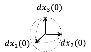
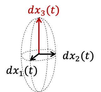
infinitesimal perturbation
D\Psi
expanded
contracted
N_+:
Dim. of unstable directions in tangent sp.
ex) one unstable direction in 3D
Jacobian matrix
Idea: Measuring 'degrees of freedom' of a chaotic system based on sensitivities to small perturbations
→ High uncertainty of prediction along this direction.
Exploiting Low Dimensionality
N_+:
Dim. of unstable directions in tangent sp.
D\Psi
Jacobian matrix
N_+ := \#\{i \mid \lambda_i > 0\}
Define
Remark positive exponent → unstable
\delta\bm{u}_n^{(i)}
\delta\bm{u}_0^{(i)}
\Psi^n
\Psi^n
|\delta\bm{u}_n^{(i)}| \approx e^{\lambda_i n} |\delta\bm{u}_0^{(i)}|
\sigma_i(A)
:
A
i
-singular value of
Lyapunov exponents:
\lambda_1 \ge \dots \ge \lambda_{N_x}
\lambda_i = \lim_{n \rightarrow \infty} \frac{1}{n} \log \sigma_i(D\Psi^n(\bm{u})).
Definition
Information on
Idea: Measuring 'degrees of freedom' of a chaotic system based on sensitivities to small perturbations
Exploiting Low Dimensionality
Ansatz (low-dimensional structure):
most geophysical flows satisfy
owing to their 'dissipative' property.
N_+ \ll N_x
Exploiting Low Dimensionality
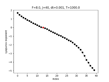
ex) 40-dim. Lorenz 96 model (chaotic toy model)
\lambda_i
i
0
unstable
stable
- Navier-Stokes equations
-
Primitive equations
(core of atmospheric model)
Other dissipative systems
N_+ = 13 \ll 40 = N_x
Lyapunov exponents
(T.+2025)
Ansatz (low-dimensional structure):
most geophysical flows satisfy
owing to their 'dissipative' property.
N_+ \ll N_x
Exploiting Low Dimensionality
Conjecture the minimum ensemble size for filter accuracy with the EnKF is
m^* = N_+ + 1.
(※ with any initial ensemble)
\Psi
\Psi
Tracking only the unstable directions
unstable direction
: critical few ensemble
Exploiting Low Dimensionality
Efficient & Accurate Weather Prediction
Conjecture the minimum ensemble size for filter accuracy with the EnKF is
m^* = N_+ + 1.
(※ with any initial ensemble)
Ansatz
N_+ \ll N_x
m \ll N_x
r
squared error
log-log
O(r^2)
EnKF with
Numerical Result
Supporting the conjecture
Numerical Result
To support the conjecture, we perform numerical experiments estimating synthetic data generated by the Lorenz 96 model.
Numerical Result
To support the conjecture, we perform numerical experiments estimating synthetic data generated by the Lorenz 96 model.
\frac{du^i}{dt} = (u^{i+1} - u^{i-2}) u^{i-1} - u^i + f
\bm{u} = (u^i)_{i=1}^{N_x} \in \mathbb{R}^{N_x}, f \in \R,
(Lorenz1996, Lorenz+1998)
u^0 = u^{N_x}, u^{-1} = u^{N_x-1}, u^{N_x + 1} = u^1.
Mimics chaotic variation of
physical quantities at equal latitudes.
u
non-linear conserving
linear dissipating
forcing
Lorenz 96 model
(i = 1, \dots, N_x),
Numerical Result
To support the conjecture, we perform numerical experiments estimating synthetic data generated by the Lorenz 96 model.
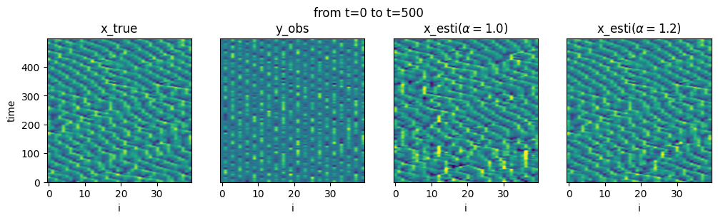
Spatio-temporal plot
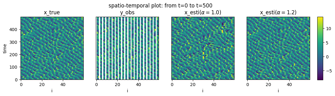
u^{i}(t)
Numerical Result
To support the conjecture, we perform numerical experiments estimating synthetic data generated by the Lorenz 96 model.
Setup (T.+2025)
obs.:
N_u=40, F=8.0
model:Lorenz96 ( )
H=I
\eta_n \sim N(0, r^2 I), r > 0
noise:
EnKF:
m = 12, 13, \dots, 18
(others are chosen appropriately)
dt = 0.01
numerical integration: RungeKutta
obs. interval:
5
N_+ = 13
N_{steps} = 72000
For each , we compute the dependency of the worst error
on .
\limsup_{n \rightarrow \infty} \mathbb{E}[|\delta_n|^2]
m
r
Numerical Result
O(r^2)
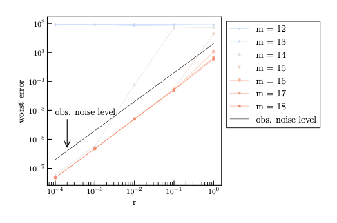
blue
(m <= N_+)
red
(m >= N_+ + 2)
gray
(m = N_+ + 1)
For each , we compute the dependency of the worst error
on → log-log plot.
m
r
r
N_+ = 13
Numerical Result
O(r^2)
O(r^2)
r
blue
(m <= N_+)
red
(m >= N_+ + 2)
gray
(m = N_+ + 1)
For each , we compute the dependency of the worst error
on → log-log plot.
m
r
N_+ = 13
Numerical Result
O(r^2)
O(r^2)
blue
(m <= N_+)
red
(m >= N_+ + 2)
gray
(m = N_+ + 1)
N_+ + 1
accurate
→ This supports the conjecture.
Inaccurate
r
For each , we compute the dependency of the worst error
on → log-log plot.
m
r
N_+ = 13
(filter accuracy)
Summary
Problem & Question
The sequential state estimation of high-dimensional chaotic systems using EnKF.
→ How many samples are required for filter accuracy?
Conjecture & Result
Determined by the unstable dimension of the dynamics.
→ Numerical evidence
→ EnKF can exploit the low-dimensional structure.
Future
Math: Proving the conjecture for dissipative systems.
Application: Spreading data assimilation in applications.
m^* = N_+ + 1
ensemble
N_+ \ll N_x
Thank you for your attention
Visit my website!
(T.+2024)
K. T. and T. Sakajo, SIAM/ASA Journal on Uncertainty Quantification, 12(4), 1315–1335,
(T.+2025)
K. T. and T. Miyoshi, EGUsphere preprint, https://egusphere.copernicus.org/preprints/2025/egusphere-2025-5144/.
References
- (T.+2024) K. T. & T. Sakajo, SIAM/ASA Journal on Uncertainty Quantification, 12(4), 1315–1335.
- (T. 2025) Kota Takeda, Error Analysis of the Ensemble Square Root Filter for Dissipative Dynamical Systems, PhD Thesis, Kyoto University, 2025.
- (Kelly+2014) D. T. B. Kelly, K. J. H. Law, and A. M. Stuart (2014), Well-posedness and accuracy of the ensemble Kalman filter in discrete and continuous time, Nonlinearity, 27, pp. 2579–260.
- (Al-Ghattas+2024) O. Al-Ghattas and D. Sanz-Alonso (2024), Non-asymptotic analysis of ensemble Kalman updates: Effective dimension and localization, Information and Inference: A Journal of the IMA, 13.
- (Tong+2016a) X. T. Tong, A. J. Majda, and D. Kelly (2016), Nonlinear stability and ergodicity of ensemble based Kalman filters, Nonlinearity, 29, pp. 657–691.
- (Tong+2016b) X. T. Tong, A. J. Majda, and D. Kelly (2016), Nonlinear stability of the ensemble Kalman filter with adaptive covariance inflation, Comm. Math. Sci., 14, pp. 1283–1313.
- (Kwiatkowski+2015) E. Kwiatkowski and J. Mandel (2015), Convergence of the square root ensemble Kalman filter in the large ensemble limit, Siam-Asa J. Uncertain. Quantif., 3, pp. 1–17.
- (Mandel+2011) J. Mandel, L. Cobb, and J. D. Beezley (2011), On the convergence of the ensemble Kalman filter, Appl.739 Math., 56, pp. 533–541.
References
-
(de Wiljes+2018) J. de Wiljes, S. Reich, and W. Stannat (2018), Long-Time Stability and Accuracy of the Ensemble Kalman-Bucy Filter for Fully Observed Processes and Small Measurement Noise, Siam J. Appl. Dyn. Syst., 17, pp. 1152–1181.
-
(Evensen2009)Evensen, G. (2009), Data Assimilation: The Ensemble Kalman Filter. Springer, Berlin, Heidelberg.
-
(Burgers+1998) G. Burgers, P. J. van Leeuwen, and G. Evensen (1998), Analysis Scheme in the Ensemble Kalman Filter, Mon. Weather Rev., 126, 1719–1724.
-
(Bishop+2001) C. H. Bishop, B. J. Etherton, and S. J. Majumdar (2001), Adaptive Sampling with the Ensemble Transform Kalman Filter. Part I: Theoretical Aspects, Mon. Weather Rev., 129, 420–436.
-
(Anderson 2001) J. L. Anderson (2001), An Ensemble Adjustment Kalman Filter for Data Assimilation, Mon. Weather Rev., 129, 2884–2903.
-
(Reich+2015) S. Reich and C. Cotter (2015), Probabilistic Forecasting and Bayesian Data Assimilation, Cambridge University Press, Cambridge.
-
(Law+2015) K. J. H. Law, A. M. Stuart, and K. C. Zygalakis (2015), Data Assimilation: A Mathematical Introduction, Springer.
References
- (Azouani+2014) A. Azouani, E. Olson, and E. S. Titi (2014), Continuous Data Assimilation Using General Interpolant Observables, J. Nonlinear Sci., 24, 277–304.
-
(Sanz-Alonso+2025), D. Sanz-Alonso and N. Waniorek (2025), Long-Time Accuracy of Ensemble Kalman Filters for Chaotic Dynamical Systems and Machine-Learned Dynamical Systems, SIAM J. Appl. Dyn. Syst., pp. 2246–2286.
-
(Biswas+2024), A. Biswas and M. Branicki (2024), A unified framework for the analysis of accuracy and stability of a class of approximate Gaussian filters for the Navier-Stokes Equations, arXiv preprint, https://arxiv.org/abs/2402.14078.
-
(T.2025) K. T. (2025), Error analysis of the projected PO method with additive inflation for the partially observed Lorenz 96 model, arXiv preprint, https://doi.org/10.48550/arXiv.2507.23199.
-
(González-Tokman+2013) C. González-Tokman and B. R. Hunt (2013) Ensemble data assimilation for hyperbolic systems, Physica D: Nonlinear Phenomena, 243(1), pp. 128–142.
-
(T.+2025) K. T. and T. Miyoshi, Quantifying the minimum ensemble size for asymptotic accuracy of the ensemble Kalman filter using the degrees of instability, EGUsphere preprint, https://egusphere.copernicus.org/preprints/2025/egusphere-2025-5144/.
Ensemble Data Assimilation in High-Dimensional Chaotic Systems: Exploiting Low-Dimensional Structures
By kotatakeda
Ensemble Data Assimilation in High-Dimensional Chaotic Systems: Exploiting Low-Dimensional Structures
20min(including Q&A)


