Random matrices
and
Quantum Chaos
Outline
- Wigner and random matrices
- Some tricks for building matrices
- Quantum chaos
Short appetizers: with relevant refernces
T. Guhr, A. Mueller-Groeling, H. A. Weidenmueller,Phys.Rept. 299, 189 (1998)
Alan Edelman and Yuyang Wang,"Random Matrix Theory and its Innovative Applications"
and as always Wikipedia and Google are your friends!
Task I
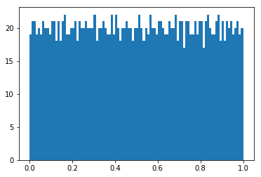
- Diagonal random matrix
a) Generate a 2000x2000 diagonal matrix with uniformly distributed random entries. The mean of the entries should be 0!
b) Calculate distribution of the eigenvalues.
(i.e. use diag() and rand() and generate a histogram)
- Symmetric full random matrix
a) Generate a 2000x2000 random symmetric matrix who's entries are drawn from the same distribution as above.
b) Calculate distribution of the eigenvalues.
- Try to fit the obtained distributions !
- If bored try other random number generators!
Cheet sheet for fitting
from scipy.optimize import curve_fit # use this for fitting
x # this is a 1D array containing sampling points of the data
y # this is a 1D array containing the data at the sampling points
# We define a function to be used for fitting
# in ths case we fit a sin
def fun(x,A,w,phi): # The signature is important!
# First argument corresponds to sampling!
return A*sin(w*x+phi) # This is just a simple sine
# with the usual parameters
#fitting is done like this
popt,pcov=curve_fit(fun,x,y)
popt # parameters of the fit go here
sqrt(diag(pcov)) # errors of the parameters are
# obtained from the covariance matrix
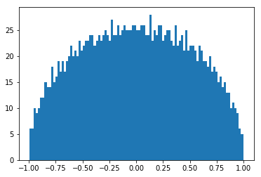
fun(x,*popt) # this will evaluate the fitted function at the sampling pointsWigner's semicircle
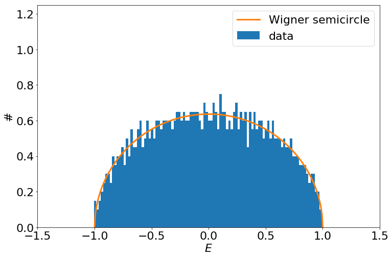
\varrho(x)=\frac{2}{\pi W^2}\sqrt{W^2-x^2}
Wigner's semicircle
- Wigner's approach for tackling spectra of large nuclei.
(Annals of Mathematics, 62 548, 1955)
- Large truly random matrices tend to have a semicircular eigenvalue distribution.
"Central limit theorem for matrices"
- Wigner's original proof concerned normally distributed matrix elements and thus he was able to match moments of the eigenvalue distribution to a semicircle.
Road to universality: Unfolding spectra
\varrho(E)\rightarrow I(E)=\displaystyle\int_{-\infty}^E \varrho(x) \mathrm{d}x\rightarrow\varepsilon_i=I(E_i)
unfolded sample
having uniform distribution
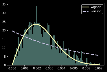
Wigner's surmise: level spacings are universal
Wigner conjectured that the distribution of the unfolded level spacings shows universal behavior...
p(s)=As^\beta e^{-B s^2}
universality class
normalization
p(s)= A e^{-s}
Integrable systems
Generic 'chaotic' systems
correlated levels
"repel" eachother
"uncorrelated" levels
can be arbitrarily close
Gaussian ensembles
-
Gaussian orthogonal ensemble (GOE),β=1
Systems with time reversal symmetry
Symmetric matrices, normally distributed real elements
-
Gaussian unitary ensemble (GUE),β=2
Generic systems without any symmetry
Hermitian matrices, normally distributed complex elements
- Gaussian symplectic ensemble (GSE),β=4
Systems with spin rotational symmetry
Symmetric matrices, normally distributed real quaternio elements
\rho(M)\sim\mathrm{e}^{-\mathrm{Tr}[MM^\dagger]}
How to unfold in practice
from scipy import interpolate # we will need interpolate data
ev=eigvalsh(H)                # get some eigenvalues

# generate the cumulative distribution of the eigenvalues
# here we use matplotlib's hist
# could use numpy's but it has no built in cumulative histogram ...
hg=hist(ev,100,cumulative=True,normed=True) # may need to play with bins

# interpolate the cumulative
# careful ! histogram generators give one more bin
ipol=interpolate.interp1d(hg[1][1:],hg[0],
                        fill_value=(0,1),bounds_error=False)
# these last options are needed to treat the edge properly


# unfolded eigenvalues
unfolded_ev=ipol(ev))
Task II
-
Generate a 2000x2000 random diagonal matrix.
- Generate 2000x2000 random matrices from Gaussian orthogonal and unitary ensembles. (If bored generate also a matrix from the symplectic ensamble!)
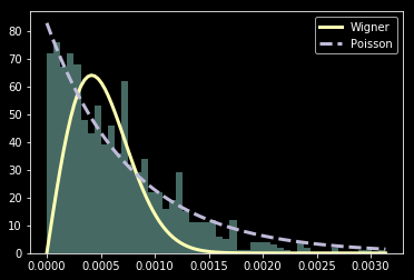
- Calculate distribution of level spacings for each matrix generated. Verify that the unfolded distribution is described by the Wigner surmise or Poisson law!
Matrix building tricks
\hat{H}=-\frac{\Delta}{2m}+V(r)
Goal: Solve the Schrödinger equation for biliard systems
Laplacian on a lattice
\psi(x)
\rightarrow\psi_x
\partial_x\psi(x)\rightarrow\frac{\psi_{x+\delta}-\psi_x}{\delta}
\partial^2_x\psi(x)\rightarrow\frac{\psi_{x+\delta}-2\psi_x+\psi_{x-\delta}}{\delta^2}
\begin{pmatrix}\ddots\\
& -2 & 1\\
& 1 & -2 & 1\\
& & 1 & -2\\
& & & & \ddots
\end{pmatrix}\cdot\begin{pmatrix}\vdots\\
\psi_{x-\delta}\\
\psi_{x}\\
\psi_{x+\delta}\\
\vdots
\end{pmatrix}
\sim\hat{H}
2D Hamiltonians
\begin{pmatrix}-4 & 1 & & & 1\\
1 & -4 & 1 & & & 1\\
& 1 & -4 & 1 & & & 1\\
& & 1 & -4 & & & & 1\\
1 & & & & -4 & 1 & & & 1\\
& 1 & & & 1 & -4 & 1 & & & 1\\
& & 1 & & & 1 & -4 & 1 & & & 1\\
& & & 1 & & & 1 & -4 & & & & 1\\
& & & & 1 & & & & -4 & 1\\
& & & & & 1 & & & 1 & -4 & 1\\
& & & & & & 1 & & & 1 & -4 & 1\\
& & & & & & & 1 & & & 1 & -4
\end{pmatrix}
y
x
Hard wall potential is realized by omitting well chosen points from the grid!
But how do I build these matrices?
diag(ones(3))
>>array([[1., 0., 0.],
         [0., 1., 0.],
         [0., 0., 1.]])
diag(ones(2),1)
>>array([[0., 1., 0.],
         [0., 0., 1.],
         [0., 0., 0.]])
kron(array([[1,0,0],
[0,1,0],
[0,0,1]]),
array([[1,2],
[3,4]])
)
>>array([[1., 2., 0., 0., 0., 0.],
[3., 4., 0., 0., 0., 0.],
[0., 0., 1., 2., 0., 0.],
[0., 0., 3., 4., 0., 0.],
[0., 0., 0., 0., 1., 2.],
[0., 0., 0., 0., 3., 4.]])Matrices with entries on
diagonals can be built with
diag()
Use kron() to build hypermatrices
Use numpy array slicing for defining the shape !!
x,y=meshgrid(...) # when defineing the lattice
                  # keep the coordinates close at hand!!

x=x.flatten()     # flatten meshgrid generated matrices
y=y.flatten()     # so we can use coordinates for indexing
...
H # let this be a Hamiltonian
  # of a regular lattice

H_potato=H[:,f(x,y)<0][f(x,y)<0,:] # bool expressions
                                   # can be used for slicing
Solving the eigensystem
va=eigenvals(H)   # only eigenvalues

va,ve=eigh(H)     # eigenvalues AND eigenvectors

# if using numpy arrays @ is the dot product
# if using numpy matrices * is the dot product
H@ve[:,i]=va[i]*ve[:,i] # the i-th eigenvector and eigenvalue satisfy this

# if coordinates of the tracked degrees of freedom
# are stored in the variables x,y

tripcolor(x,y,abs(ve[:,i])**2) # this will visualize the i-th eigenvector
Sparse matrices
# these are modules to deal with sparse matrices
import scipy.sparse as ss
import scipy.sparse.linalg as sl

# matrix building functions have sparse alternatives
idL=ss.eye(L)                    # identity
odL=ss.diags(ones(L-1),1,(L,L))  # off diagonal

ss.kron(A,B) # kron is also here

# cut region of interest
Hsliced=H[:,slice][slice,:]            # slicing works if sparse
Hsliced=(H.tocsr())[:,slice][slice,:]  # csr format is used
                                       # casting from other formats
                                       # might be needed

# Some (strictly not all) eigenvalues can be obtained
# Lanczos and Arnoldi algorithms are used in the background
va,ve=sl.eigsh(Hsliced,30,sigma=0.5)   # this gets 30 eigenvalues
                                       # and eigenvectors from around 0.5
Task III
- Generate Hamiltonian of a 2D particle on a lattice in a rectangle region.
- Generate Hamiltonian in an arbitrary potato shaped region.
- Find lowest couple of eigenvalues (eigenvectors as well if bored)
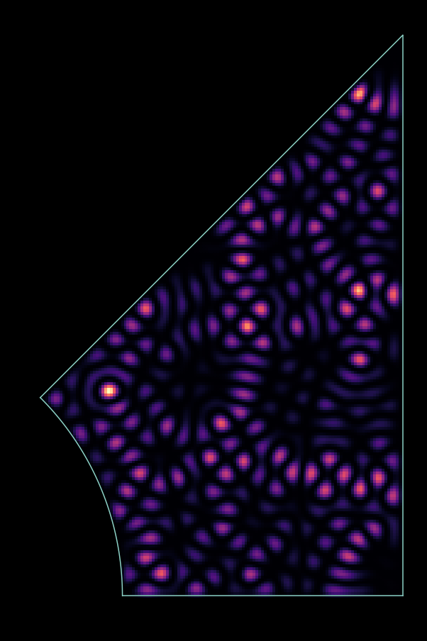
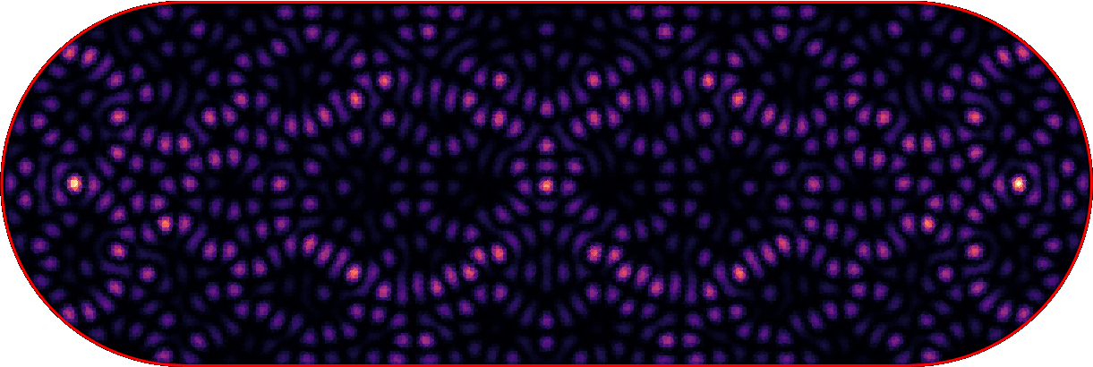
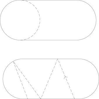
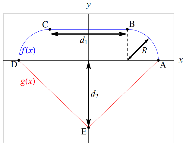
- Investigate the Sinai billiard in the integrable (R=0) and chaotic limit (R>0).
a) Generate a Hamiltonian for the system in the picture.
(give max 4000x4000 matrices to eig() )
b) Calculate unfolded eigenvalues.
c) Calculate level spacing distribution for
both cases.

Extra: explore other billiards
- Elipse
- Bunimovich stadium
- Diamond
- Add magnetic field for GUE biliards

- get rid of all rotational and mirror symmetries
- go for larger grids with sparse matrices
Quantum Chaos -> Wigner surmise
R=0
R=1
Some considerations
- Discretization can make integrable seem chaotic.
(Wigner instead of Poisson) - Spurious symmetries can make chaotic seem integrable. (Poisson instead of Wigner)
- In order to get rid of artifacts grid may need to be large.
- Adaptive grid can help discretization error.
- Sparse matrices and Lanczos algorithm can be used to get reasonable amount of data in reasonably short time.
Random matrices and Quantum Chaos
By László Oroszlány


