Double-bracket flow quantum algorithm for diagonalization
Marek Gluza
NTU Singapore
slides.com/marekgluza

New quantum algorithm for diagonalization
\hat H \mapsto \hat \mathcal H_\ell = \hat \mathcal U_\ell^\dagger \hat H \hat\mathcal U_\ell
\partial_\ell \hat \mathcal H_\ell = [[A(\hat \mathcal H_\ell),B(\hat \mathcal H_\ell)], \hat \mathcal H_\ell]
no qubit overheads
no controlled-unitaries
0
0
0
0
C
0
0
0
0
Simple
=
Easy
Doesn't spark joy :(
New quantum algorithm for diagonalization
\hat H \mapsto \hat \mathcal H_\ell = \hat \mathcal U_\ell^\dagger \hat H \hat\mathcal U_\ell
\partial_\ell \hat \mathcal H_\ell = [[A(\hat \mathcal H_\ell),B(\hat \mathcal H_\ell)], \hat \mathcal H_\ell]
building useful quantum algorithms
new approach to preparing useful states
building useful variational circuits
tons of fun maths in the appendix
no qubit overheads
no controlled-unitaries
0
0
0
0
New quantum algorithm for diagonalization
\hat H \mapsto \hat \mathcal H_\ell = \hat \mathcal U_\ell^\dagger \hat H \hat\mathcal U_\ell
\partial_\ell \hat \mathcal H_\ell = [[A(\hat \mathcal H_\ell),B(\hat \mathcal H_\ell)], \hat \mathcal H_\ell]
0
0
0
0
\hat D_s(\hat J) = \prod_{\mu\in\{0,1\}^{\times L}} \hat Z_\mu e^{-i s \hat J/ \text{dim}(\hat J)} \hat Z_\mu
\hat C_s(\hat J) = \hat D_{\sqrt{2s}}(\hat J)^\dagger e^{i\sqrt{2s}\hat J}\hat D_{\sqrt{2s}}(\hat J)e^{-i\sqrt{2s}\hat J}
\hat V_k = \hat V_{k-1}\hat C_s(\hat J_{k-1})
\hat J_{k-1} = \hat V_{k-1}^\dagger \hat H \hat V_{k-1}
1) Dephasing
2) Group commutator
3) Frame shifting

What have
condensed-matter theorists
been up to in the 90's?
BTW: For the next 2 years I will be working on theory support for prof. Rainer Dumke as NTU PPF (super-conducting qubits, tomography zoo, proof-of-principle quantum algorithms...)
Research assistant "quantum engineer" positions available
(python, mathematica, Qiskit)
\hat H
\hat \mathcal H_\ell = \hat \mathcal U_\ell^\dagger \hat H \hat\mathcal U_\ell
\partial_\ell \hat \mathcal H_\ell = [\hat \mathcal W_\ell, \hat \mathcal H_\ell]
\hat \mathcal W_\ell = [\Delta(\hat \mathcal H_\ell),\sigma(\hat \mathcal H_\ell)]
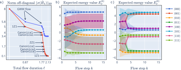
\partial_\ell \|\sigma(\hat \mathcal H_\ell)\|_{\text{HS}}^2 = -2\|\hat \mathcal W_\ell\|_{\text{HS}}^2
\Delta(\hat \mathcal H_\ell)
\sigma(\hat \mathcal H_\ell)
Głazek-Wilson-Wegner flow
GWW flow equation
Flow duration
GWW flow unitary
Flowed Hamiltonian
Input Hamiltonian
\hat\mathcal U_\ell
\ell
Canonical bracket
GWW flow monotonicity
Restriction to off-diagonal
Restriction to diagonal
as a quantum algorithm
\hat H
\hat \mathcal H_\ell = \hat \mathcal U_\ell^\dagger \hat H \hat\mathcal U_\ell
\partial_\ell \hat \mathcal H_\ell = [\hat \mathcal W_\ell, \hat \mathcal H_\ell]
\hat \mathcal W_\ell = [\Delta(\hat \mathcal H_\ell),\sigma(\hat \mathcal H_\ell)]
\Delta(\hat \mathcal H_\ell)
\sigma(\hat \mathcal H_\ell)
Głazek-Wilson-Wegner flow
GWW flow equation
Flow duration
GWW flow unitary
Flowed Hamiltonian
Input Hamiltonian
\hat\mathcal U_\ell
\ell
Canonical bracket
GWW flow monotonicity
Restriction to off-diagonal
Restriction to diagonal
\hat H
\hat \mathcal H_\ell = \hat \mathcal U_\ell^\dagger \hat H \hat\mathcal U_\ell
\partial_\ell \hat \mathcal H_\ell = [\hat \mathcal W_\ell, \hat \mathcal H_\ell]
\hat \mathcal W_\ell = [\Delta(\hat \mathcal H_\ell),\sigma(\hat \mathcal H_\ell)]
\partial_\ell \|\sigma(\hat \mathcal H_\ell)\|_{\text{HS}}^2 = -2\|\hat \mathcal W_\ell\|_{\text{HS}}^2
\Delta(\hat \mathcal H_\ell)
\sigma(\hat \mathcal H_\ell)
Głazek-Wilson-Wegner flow
GWW flow equation
Flow duration
GWW flow unitary
Flowed Hamiltonian
Input Hamiltonian
\hat\mathcal U_\ell
\ell
Canonical bracket
GWW flow monotonicity
Restriction to off-diagonal
Restriction to diagonal
as a quantum algorithm
\hat \mathcal W_\ell = [\Delta(\hat \mathcal H_\ell),\sigma(\hat \mathcal H_\ell)]
\partial_\ell \|\sigma(\hat \mathcal H_\ell)\|_{\text{HS}}^2 = -2\|\hat \mathcal W_\ell\|_{\text{HS}}^2 \le 0
Głazek-Wilson-Wegner flow
GWW flow monotonicity
as a quantum algorithm
What's going on?
Double-bracket flow
Unitary
Satisfies a generalization of the Heisenberg equation
\hat \mathcal H_\ell = \hat \mathcal U_\ell^\dagger \hat H \hat\mathcal U_\ell
\partial_\ell \hat \mathcal H_\ell = [[A(\hat \mathcal H_\ell),B(\hat \mathcal H_\ell)], \hat \mathcal H_\ell]
\hat\mathcal U_\ell
GWW is a particular example
\partial_\ell \hat \mathcal H_\ell = [[\Delta(\hat \mathcal H_\ell),\sigma(\hat \mathcal H_\ell)], \hat \mathcal H_\ell]
transformation of
\hat H
\hat H_s = e^{s \hat W^{(Z)}} \hat H e^{-s \hat W^{(Z)}}
\hat W^{(Z)} = [\Delta^{(Z)}(\hat H), \hat H ],
\partial_s \|\sigma(\hat H_s)\|_{\text{HS}}^2 = -2\langle \hat W^{(Z)},\hat W\rangle_{\text{HS}}
\Delta^{(Z)}(\hat H) \text{ - diagonal}
Variational double-bracket flows
that are diagonalizing

\partial_\ell \|\sigma(\hat \mathcal H_\ell)\|_{\text{HS}}^2 = -2\|\hat \mathcal W_\ell\|_{\text{HS}}^2 \le 0
antihermitian
unitary
\left(i\hat H\right)^\dagger = -i \hat H
How to understand the continuous flow?
\hat H_1 = e^{s \hat W_1} \hat H e^{-s \hat W_1}
\hat W_1 = [\Delta(\hat H),\sigma(\hat H)]
\hat W_k = [\Delta(\hat H_{k-1}),\sigma(\hat H_{k-1})]
\hat H_k = e^{s \hat W_k} \hat H_{k-1} e^{-s \hat W_k}

\hat H_\text{TFIM} = \sum_{i=1}^{L-1}\hat X_i\hat X_{i+1}+\sum_{i=1}^L \hat Z_i
Piece-wise constant discretization
\hat W_k = [\Delta(\hat H_{k-1}),\sigma(\hat H_{k-1})]
\hat H_k = e^{s \hat W_k} \hat H_{k-1} e^{-s \hat W_k}
\text{If we want } U_\ell \text{ then set } s = \ell / N \text{ and } N\rightarrow \infty
\text{{\bf Prop.} This converges point-wise:}
\partial_\ell \hat \mathcal H_\ell = [\hat \mathcal W_\ell, \hat \mathcal H_\ell]
\hat \mathcal W_\ell = [\Delta(\hat \mathcal H_\ell),\sigma(\hat \mathcal H_\ell)]
Piece-wise constant discretization
\hat W_k = [\Delta(\hat H_{k-1}),\sigma(\hat H_{k-1})]
\hat H_k = e^{s \hat W_k} \hat H_{k-1} e^{-s \hat W_k}
Notation for later:
\hat J_k = \hat V_k^\dagger \hat H \hat V_k
\hat V_k\approx e^{-s\hat W_1}\;e^{-s\hat W_2}\ldots e^{-s\hat W_k}
Quantum algorithm needs to be aiming to approximate rather than directly implement
How to quantum?
Group commutator
\hat H \mapsto \hat \mathcal H_\ell = \hat \mathcal U_\ell^\dagger \hat H \hat\mathcal U_\ell
\partial_\ell \hat \mathcal H_\ell = [[A(\hat \mathcal H_\ell),B(\hat \mathcal H_\ell)], \hat \mathcal H_\ell]
0
0
0
0
Want
\hat H_1 = e^{s \hat W_1} \hat H e^{-s \hat W_1}
\hat W_1 = [\Delta(\hat H),\sigma(\hat H)]
e^{is\Delta(\hat H)}e^{is\hat H}e^{-is\Delta(\hat H)}e^{-is\hat H}= e^{-\frac12 s^2[\Delta(\hat H),\sigma(\hat H)]} +\hat E^\text{(GC)}
New bound
\|\hat E^\text{(GC)}\| \le 4\|\hat H\|\,\|[\Delta(\hat H),\sigma(\hat H)]\| s^3
Group commutator
\hat H \mapsto \hat \mathcal H_\ell = \hat \mathcal U_\ell^\dagger \hat H \hat\mathcal U_\ell
\partial_\ell \hat \mathcal H_\ell = [[A(\hat \mathcal H_\ell),B(\hat \mathcal H_\ell)], \hat \mathcal H_\ell]
0
0
0
0
Want
\hat H_1 = e^{s \hat W_1} \hat H e^{-s \hat W_1}
\hat W_1 = [\Delta(\hat H),\sigma(\hat H)]
e^{is\Delta(\hat H)}e^{is\hat H}e^{-is\Delta(\hat H)}e^{-is\hat H}= e^{-\frac12 s^2[\Delta(\hat H),\sigma(\hat H)]} +\hat E^\text{(GC)}
How to get ?
\hat D_s(\hat H) \approx e^{is\Delta(\hat H)}
\hat C_s(\hat J) = \hat D_{\sqrt{2s}}(\hat J)^\dagger \; e^{i\sqrt{2s}\hat J}\; \hat D_{\sqrt{2s}}(\hat J)\; e^{-i\sqrt{2s}\hat J}
\approx e^{-s \hat W(\hat J)}
New quantum algorithm for diagonalization
\hat H \mapsto \hat \mathcal H_\ell = \hat \mathcal U_\ell^\dagger \hat H \hat\mathcal U_\ell
\partial_\ell \hat \mathcal H_\ell = [[A(\hat \mathcal H_\ell),B(\hat \mathcal H_\ell)], \hat \mathcal H_\ell]
0
0
0
0
\hat D_s(\hat J) = \prod_{\mu\in\{0,1\}^{\times L}} \hat Z_\mu e^{-i s \hat J/D} \hat Z_\mu
\hat C_s(\hat J) = \hat D_{\sqrt{2s}}(\hat J)^\dagger \; e^{i\sqrt{2s}\hat J}\;\hat D_{\sqrt{2s}}(\hat J)\;e^{-i\sqrt{2s}\hat J}
\hat V_k = \hat V_{k-1}\hat C_s(\hat J_{k-1})
\hat J_{k-1} = \hat V_{k-1}^\dagger \hat H \hat V_{k-1}
1) Dephasing
2) Group commutator
3) Frame shifting
\hat H
\hat \mathcal H_\ell = \hat \mathcal U_\ell^\dagger \hat H \hat\mathcal U_\ell
\partial_\ell \hat \mathcal H_\ell = [\hat \mathcal W_\ell, \hat \mathcal H_\ell]
\hat \mathcal W_\ell = [\Delta(\hat \mathcal H_\ell),\sigma(\hat \mathcal H_\ell)]
\partial_\ell \|\sigma(\hat \mathcal H_\ell)\|_{\text{HS}}^2 = -2\|\sigma(\hat \mathcal W_\ell)\|_{\text{HS}}^2
\Delta(\hat \mathcal H_\ell)
\sigma(\hat \mathcal H_\ell)
Głazek-Wilson-Wegner flow
GWW flow equation
Flow duration
GWW flow unitary
Flowed Hamiltonian
Input Hamiltonian
\hat\mathcal U_\ell
\ell
Canonical bracket
GWW flow monotonicity
Restriction to off-diagonal
Restriction to diagonal
Dephasing is a unitary mixing channel:
\Delta(\hat \mathcal H_\ell)= \frac 1 D \sum_{\mu\in\{0,1\}^{\times L}} \hat Z_\mu \hat\mathcal H_\ell \hat Z_\mu
as a quantum algorithm
1,
1,
1,
1,
0,
0,
0,
0
What I mean by phase flips
\mu = (
)
N
S
N
S
N
S
N
S
\hat Z
\mathbb 1
\mathbb 1
\otimes
\otimes
\otimes
\otimes
\otimes
\otimes
\otimes
\hat Z
\hat Z
\hat Z
\mathbb 1
\mathbb 1
0,
1,
0,
1,
0,
0,
0,
1
What I mean by phase flips
\mu = (
)
1
\otimes
\mathbb 1
\otimes
\mathbb 1
\otimes
\hat Z
\otimes
1
\otimes
\mathbb 1
\otimes
\hat Z
\otimes
\hat Z
N
S
N
S
N
S
Evolution under dephased generators
\hat H \mapsto \hat \mathcal H_\ell = \hat \mathcal U_\ell^\dagger \hat H \hat\mathcal U_\ell
\partial_\ell \hat \mathcal H_\ell = [[A(\hat \mathcal H_\ell),B(\hat \mathcal H_\ell)], \hat \mathcal H_\ell]
0
0
0
0
\hat Z_\mu e^{-i s \hat J} \hat Z_\mu = e^{-is \hat Z_\mu \hat J\hat Z_\mu}
\hat D_s(\hat J) \approx \prod_{\mu\in R} \hat Z_\mu e^{-i s \hat J/D} \hat Z_\mu
We can make it efficient:
\Delta(\hat J)= \frac 1 {\dim (\hat J)} \sum_{\mu\in\{0,1\}^{\times L}} \hat Z_\mu \hat J \hat Z_\mu
R \subseteq \{0,1\}^{\times L}
Use unitarity
and repeat many times
New quantum algorithm for diagonalization
\hat H \mapsto \hat \mathcal H_\ell = \hat \mathcal U_\ell^\dagger \hat H \hat\mathcal U_\ell
\partial_\ell \hat \mathcal H_\ell = [[A(\hat \mathcal H_\ell),B(\hat \mathcal H_\ell)], \hat \mathcal H_\ell]
0
0
0
0
\hat D_s(\hat J) = \prod_{\mu\in\{0,1\}^{\times L}} \hat Z_\mu e^{-i s \hat J/D} \hat Z_\mu
\hat C_s(\hat J) = \hat D_{\sqrt{2s}}(\hat J)^\dagger \;e^{i\sqrt{2s}\hat J}\;\hat D_{\sqrt{2s}}(\hat J)\;e^{-i\sqrt{2s}\hat J}
\hat V_k = \hat V_{k-1}\hat C_s(\hat J_{k-1})
\hat J_{k-1} = \hat V_{k-1}^\dagger \hat H \hat V_{k-1}
1) Dephasing
2) Group commutator
3) Frame shifting
How well does it work?

Variational flow example
Notice the steady increase of diagonal dominance.


Variational vs. GWW flow
Notice that degeneracies limit GWW diagonalization but variational brackets can lift them.

GWW for 9 qubits
Notice the spectrum is almost converged.


GWW for 9 qubits
Notice that some of them are essentially eigenstates!
Runtime
- are you running the full scheme?
\text{{\bf Prop.} The prescription converges to GWW } \\ \|\hat V_N -\hat \mathcal U_\ell\|\le O\left(e^{16 \|\hat H\|^2\ell} \sqrt{\frac \ell N}\right)
- number of queries assuming worst-case
\mathcal N(N) \sim 2^{N L}
Runtime
- are you running heuristics?
1) Not
s = \ell / N
s_1,\ldots, s_N
but optimize durations

2) It's not necessary to Hamiltonian simulate
e^{-s\hat W}
3) It's possible to Hamiltonian simulate
\hat V^\text{(pGGW)} = e^{-s_1 \hat W_1}\ldots e^{-s_5 \hat W_5}
4) Use approximate dephasing
5) Use variational brackets
Each of these reduces the runtime
\mathcal N(N) \sim poly(N) exp(L)
\mathcal N(N) \sim poly(N,L)
How does it work again?
Quantum algorithm for diagonalization
\hat H \mapsto \hat \mathcal H_\ell = \hat \mathcal U_\ell^\dagger \hat H \hat\mathcal U_\ell
\partial_\ell \hat \mathcal H_\ell = [[A(\hat \mathcal H_\ell),B(\hat \mathcal H_\ell)], \hat \mathcal H_\ell]
0
0
0
0
\hat D_s(\hat J) = \prod_{\mu\in\{0,1\}^{\times L}} \hat Z_\mu e^{-i s \hat J/ \dim(\hat J)} \hat Z_\mu
\hat C_s(\hat J) = \hat D_{\sqrt{2s}}(\hat J)^\dagger\; e^{i\sqrt{2s}\hat J}\;\hat D_{\sqrt{2s}}(\hat J)\;e^{-i\sqrt{2s}\hat J}
\hat V_k = \hat V_{k-1}\hat C_s(\hat J_{k-1})
\hat J_{k-1} = \hat V_{k-1}^\dagger \hat H \hat V_{k-1}
1) Dephasing
2) Group commutator
3) Frame shifting
\hat V_k = \hat C_s(\hat J_{1})\; \hat C_s(\hat J_{2})\ldots \hat C_s(\hat J_{k-1}) \approx e^{-s \hat W_1}\;e^{-s \hat W_2}\ldots e^{-s \hat W_{k-1}}
Recursion unfolded
\hat W_1 = [\Delta(\hat H), \sigma(\hat H)]
\hat W_2 = [\Delta(\hat H_1), \sigma(\hat H_1)]
\ldots
What else is there?
Linear programming
Matching optimization
Diagonalization
Sorting
QR decomposition
Toda flow
Material science?
0
0
0
0
C
|\psi(t)\rangle = e^{-it \hat H}|\psi(0)\rangle
How to compute it on a laptop?
How to compute it on a quantum computer?
Hamiltonian simulation
|\psi(t)\rangle = e^{-it \hat H}|\psi(0)\rangle
How to compute it on a quantum computer?
Use quantum algorithms 'Hamiltonian simulation'
Trotter-Suzuki
Linear combination of unitaries
Qubitization
Randomized compiler
Hamiltonian simulation
Gaussian quantum simulators


Trotter-Suzuki decomposition
\|\hat E\| = \|e^{-it(\hat H_X +\hat H_Z)} - \left(e^{-i\frac tN \hat H_X}e^{-i\frac tN \hat H_Z}\right)^N\|
\le \frac{t^2}N\|[\hat H_X,\hat H_Z]\|
Why does it work?
BCH formula
e^{-it( \hat H_X +\hat H_Z)}=e^{-it\hat H_X }e^{-it\hat H_Z}e^{-i\frac {t^2}2[\hat H_X ,\hat H_Z]}\ldots
\|\mathbb 1 - e^{-i\frac {t^2}2[\hat H_X ,\hat H_Z]}\| \le \frac {t^2}2 \|[ \hat H_X ,\hat H_Z]\|
Conclusion: For short evolution time we're happy
How to implement Trotter-Suzuki?
e^{-it\hat H_X}=\prod_{i=1}^{L-1}e^{-it X_iX_{i+1} }
g_X(i) = e^{-itX_i X_{i+1}}
g_Z(i) = e^{-itZ_i }
Use Solovay-Kitaev algorithm to compile these gates but usually they are the primitive gates
(e^{-i\frac tN \hat H_X}e^{-i\frac tN \hat H_Z})^N{|0\rangle}^{\otimes L}
0
0
0
0
Hamiltonian simulation
0
0
0
0
0
0
0
0
C

Most sophisticated theoretical methods use
controlled-unitary operations
Exercise: Local error bound
Q_x = e^{i(1-x)A}e^{i(1-x)B}e^{ix(A+B)}
Q_1 = e^{i(A+B)}
Q_0 = e^{i A}e^{i B}
\partial_x Q_x = e^{i(1-x)A}\left(-A-B+ A_B+B\right)e^{i(1-x)B} e^{ix(A+B)}
A_B = e^{i(1-x)B}A e^{-i(1-x)B} = A + i e^{i\xi_x B}[A,B] e^{-i\xi_x B}
\|Q_0-Q_1\| =\| \int_0^1 dx \partial_x Q_x\| = \|[A,B]\|
Exercise: Non-commutative identity
X^m - Y^m = \sum_{j=0}^{m-1}X^{m-1-j}(X-Y)Y^j
\le \sum_{j=0}^{N-1}\|e^{-i (N-1-j)\frac tN \hat H_X}(e^{-i\frac tN \hat H_X}-e^{-i\frac tN \hat H_Z})e^{-ij\frac tN \hat H_Z}\|
\|e^{-it(\hat H_X +\hat H_Z)} - \left(e^{-i\frac tN \hat H_X}e^{-i\frac tN \hat H_Z}\right)^N\|
\le \sum_{j=0}^{N-1}\|e^{-i \frac tN \hat H_X}-e^{-i\frac tN \hat H_Z}\| \le \frac{t^2}N \|[H_X,H_Z]\|
cf.:
x^m -y ^m = (x-y)\sum_{j=0}^{m-1}x^{m-1-j}y^j
Application to physics:
Version 2022 shortened: Double-bracket flow quantum algorithm for diagonalization
By Marek Gluza


