Active Tactile Exploration for Dynamic Pose and Shape Estimation

Ethan K. Gordon, Bruk Baraki, Hien Bui, Michael Posa

https://dairlab.github.io/activetactile

Supported by: NSF CAREER Award FRR-2238480, RAI Institute

ethankg@seas.upenn.edu

RESULTS

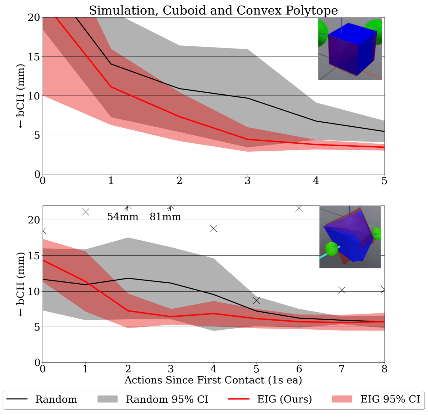
• Bidirectional Chamfer Distance (bCH) Evaluation Metric
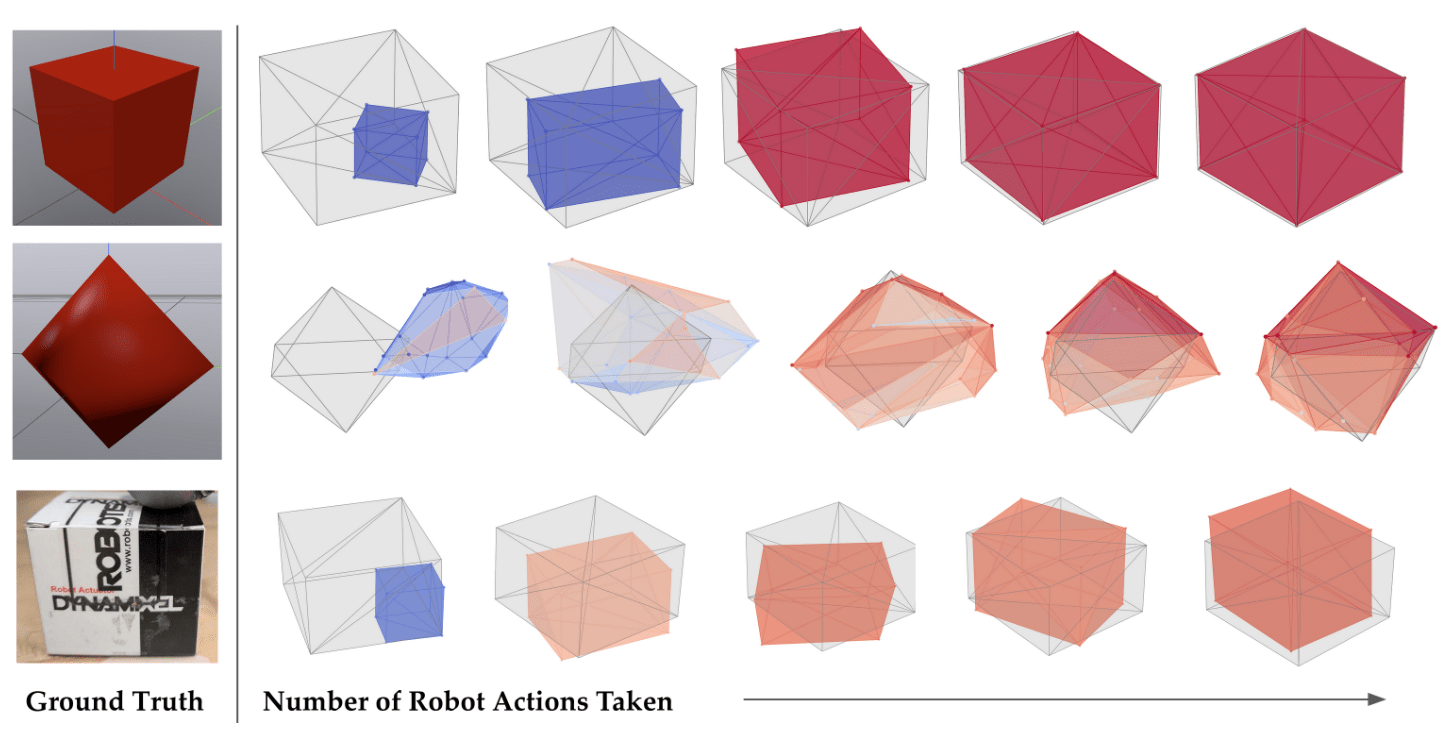
• (Left) Simulated results for cuboid and polytope parameterizations.
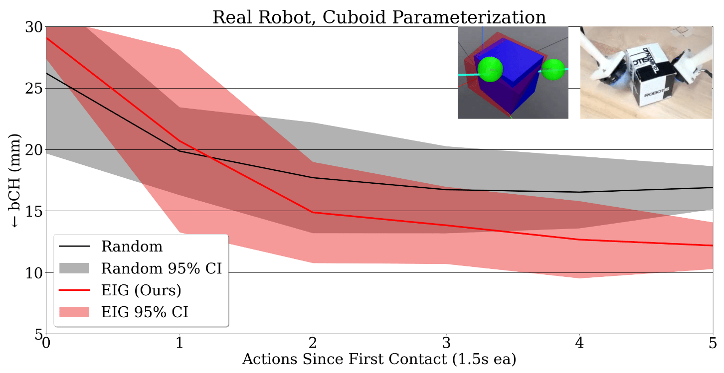
• (Top Right) Real robot results
• Significant improvement over object-directed actions from random approach directions.
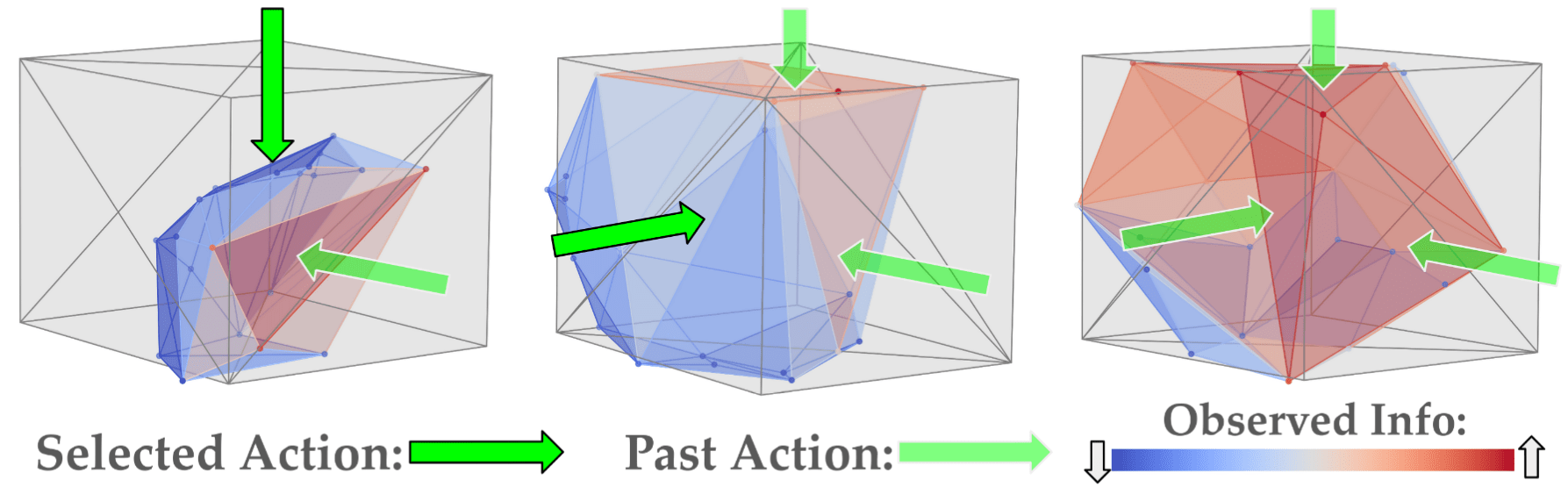
• (Bottom Right) Example learning curves. Observed information increases with more data.

EXPERIMENT SETUP

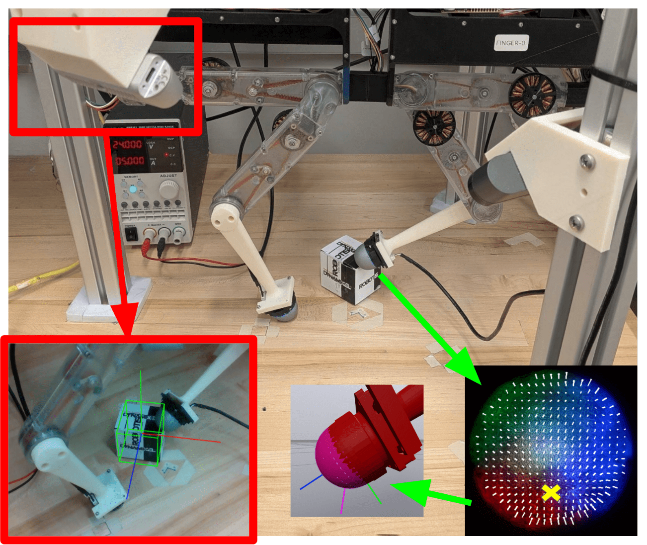
• Trifinger Robot
• Densetact 2.0 (Do, 2023)
• Contact Boolean \(c_t\) and Normal \(\hat{n}_t\) are computed with Optical Flow and a Helmholz-Hodge Decomposition
• Realsense for Ground-Truth only

INTRODUCTION

• Each action: 1s trajectory towards the current guess
• Baseline (Random): Randomize approach direction
• EIG (Ours): Choose the approach to maximize EIG, sampling-based optimization with Gaussian Cross-Entropy Method

• Learning a physical model online can improve data efficiency, predictability, and reuse between tasks.
• Previous Tactile System Identification Work: Static Objects and/or Strong Shape Priors and/or 2D
• Learning: a violation-implicit loss function penalizes physical constraint violation while avoiding the numerical stiffness inherent in rigid-body contact.
• We learn cuboid and convex polyhedra with less than 10s of randomly collected data.
• Exploration: maximizing Expected Info Gain (EIG) leads to significantly faster learning.

Only tactile data is used to find the pose and geometry of an arbitrary dynamic convex object.

METHOD AND FRAMEWORK

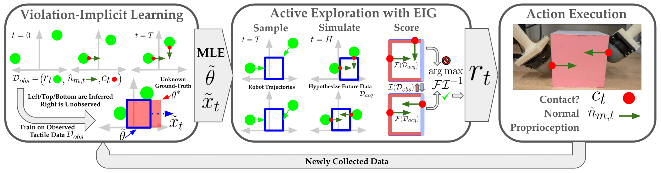
• Learning Difficulty: gradients of dynamics \(f\) are near-0 or near-\(\infty\), which is not amenable to learning.
• Solution: add inner optimization over contact forces \(\lambda\). Trade-off: solving a (fast) QP each gradient step for better gradients.

\(\sum_t \mathbb{P}(m_t | \theta, x_t) + ||x_t - f_\theta(x_{t-1}, \lambda)||^2\)

Where \(\lambda = \min g_\theta(x, \lambda)\)

\(\mathcal{L} = \sum_t \min_\lambda\mathbb{P}(m_t | \theta, x_t) + ||x_t - f_\theta(x_{t-1})||^2 + g_\theta(x, \lambda)\)

Physics Constrained MLE with Trajectory Optimization

Violation-Implicit Loss

• Observed Information: empirical variance of loss gradient

\(\mathcal{I} = \sum_{m_t} \nabla\mathcal{L}(\theta, x_T) \left(\nabla \mathcal{L}(\theta, x_T\right)^T\)

Measurements \(m_t\)

• Fisher Information: expected variance given future \(m_t\)

\(\mathcal{F} = \mathbb{E}_{m_t}\left[\nabla\mathcal{L}(\theta, x_T) \left(\nabla \mathcal{L}(\theta, x_T\right)^T\right]\)

• Sample future actions, Simulate to estimate \(\mathcal{F}\), then maximize Expected Information Gain (EIG)

\(EIG := \log\det\left(\mathcal{F}\mathcal{I}^{-1} + \mathbf{I}\right)\)