SIGNATURES OF RELIC QUANTUM
NONEQUILIBRIUM
Nicolas Graeme Underwood
PhD Thesis Defense
Department of Physics and Astronomy
Clemson University
26th April 2019
Why study the foundations of quantum mechanics?
- Because nearly 100 years after the second quantum revolution, the measurement problem still exists.
- Because it is coming into ever sharper focus with the maturity of disciplines like cosmology.
- Because it contains the mystery of operationalism vs. realism, and resultant effects like contextuality.
- Because progress in our most advanced quantum theories (quantum gravity) has been proving difficult.
- Because the field is under-developed.
- Because quantum relaxation explains quantum probabilities
This is a de Broglie-Bohm system
It mimics quantum probabilities through the motion of ensembles.
Every system has a definite position (more accurately configuration).
It is deterministic, time reversible, it does not include quantum state collapses or other non-unitary behavior.
The measurement theory compellingly accounts for contextuality.
And of course quantum relaxation...
And of course quantum relaxation...
In the de Broglie-Bohm theory I see two genuinely compelling factors:
1) The measurement theory - Naturally includes observers in the system. Naturally accounts for contextuality. Gives a compelling reason why quantum state collapse is included in textbook quantum mechanics
2) Quantum relaxation - Spontaneously relaxes to quantum probabilities. (It is amazing that nobody realized this sooner.)
I would argue that many of the details are far from being finalized, however.
In the de Broglie-Bohm theory I see two genuinely compelling factors:
I would argue that many of the details are far from being finalized, however.
I prefer to ask the question ‘What is required of a theory so that it retains the classical notion of thermodynamic relaxation, but instead relaxes to reproduce quantum probabilities?’
1) The measurement theory - Naturally includes observers in the system. Naturally accounts for contextuality. Gives a compelling reason why quantum state collapse is included in textbook quantum mechanics
2) Quantum relaxation - Spontaneously relaxes to quantum probabilities. (It is amazing that nobody realized this sooner.)
The iRelax Framework
Ingredient 1) A state-space:
Ingredient 2) A law of evolution:
Ingredient 3) An equilibrium distribution (max entropy):
Ingredient 4) A measure for information (entropy):
Ingredient 5) A statement of information (entropy) conservation
Ingredient 6) A reasonable mechanism by which entropy de facto rises
\Omega
\dot{x}
\rho_\text{eq}(x)
S
Ingredient 1) A state-space:
The space of all possible states the ‘system’ may hold. The system is defined with reference to the state-space. By a state-space, only the usual notion is meant. A single coordinate x in the state-space should correspond to a single system state. Each individual system should occupy a single state x at any time t.
The iRelax Framework
Ingredient 1) A state-space:
Ingredient 2) A law of evolution:
Ingredient 3) An equilibrium distribution (max entropy):
Ingredient 4) A measure for information (entropy):
Ingredient 5) A statement of information (entropy) conservation
Ingredient 6) A reasonable mechanism by which entropy de facto rises
\Omega
\dot{x}
\rho_\text{eq}(x)
S
Ingredient 2) A law of evolution:
The law of evolution should entirely determine the future evolution of the system, given its current state-space coordinate.
Actually, this requirement may not be necessary. It may already follow as a result of entropy information conservation, ingredient 5. (See later on missing link)
The iRelax Framework
Ingredient 1) A state-space:
Ingredient 2) A law of evolution:
Ingredient 3) An equilibrium distribution (max entropy):
Ingredient 4) A measure for information (entropy):
Ingredient 5) A statement of information (entropy) conservation
Ingredient 6) A reasonable mechanism by which entropy de facto rises
\Omega
\dot{x}
\rho_\text{eq}(x)
S
As entropy is conserved (ingredient 5), any distribution with a uniquely maximum entropy must be conserved by the law of evolution, ingredient 1. The distribution of
maximum entropy/least information may therefore be regarded as a stable equilibrium distribution, hence the notation \(\rho_\text{eq}(x)\).
Ingredient 3) An equilibrium distribution (max entropy):
The iRelax Framework
Ingredient 1) A state-space:
Ingredient 2) A law of evolution:
Ingredient 3) An equilibrium distribution (max entropy):
Ingredient 4) A measure for information (entropy):
Ingredient 5) A statement of information (entropy) conservation
Ingredient 6) A reasonable mechanism by which entropy de facto rises
\Omega
\dot{x}
\rho_\text{eq}(x)
S
Ingredient 3 and ingredient 4 must be consistent with each other. Later, entropy will be defined with respect to the equilibrium distribution.
Ingredient 4) A measure for information (entropy):
The iRelax Framework
Ingredient 1) A state-space:
Ingredient 2) A law of evolution:
Ingredient 3) An equilibrium distribution (max entropy):
Ingredient 4) A measure for information (entropy):
Ingredient 5) A statement of information (entropy) conservation
Ingredient 6) A reasonable mechanism by which entropy de facto rises
\Omega
\dot{x}
\rho_\text{eq}(x)
S
Ingredient 5) A statement of information (entropy) conservation
Information conservation is defined with respect to information measure, ingredient 4. It must be consistent with the law of evolution, ingredient 2. Information conservation will usually be expressed in terms of a (modified) Liouville theorem.
The iRelax Framework
Ingredient 1) A state-space:
Ingredient 2) A law of evolution:
Ingredient 3) An equilibrium distribution (max entropy):
Ingredient 4) A measure for information (entropy):
Ingredient 5) A statement of information (entropy) conservation
Ingredient 6) A reasonable mechanism by which entropy de facto rises
\Omega
\dot{x}
\rho_\text{eq}(x)
S
Since by ingredient 5 the exact entropy is conserved, it may only rise in effect through some limitation of experiment. Various means by which this comes about are discussed below. Ingredient 6 is included as it is useful to consider the qualitative causes of relaxation. This aids for example in the recognition of relaxation taking place, and the identification of any potential barriers to full relaxation.
Ingredient 6) A reasonable mechanism by which entropy de facto rises
Discrete iRelax theories
| Ingredient | |
|---|---|
| 1) State-space | |
| 2) Law of evolution | |
| 3) Equilibrium distribution | |
| 4) Information measure | |
| 5) Information conservation | |
| 6) De facto entropy rise |
Discrete iRelax theories
| Ingredient | |
|---|---|
| 1) State-space | |
| 2) Law of evolution | |
| 3) Equilibrium distribution | |
| 4) Information measure | |
| 5) Information conservation | |
| 6) De facto entropy rise |
E
A
B
C
D
E
A
B
C
D
E
A
B
C
D
E
A
B
C
D
\Omega = \{A,B,C,...\}
Discrete iRelax theories
| Ingredient | |
|---|---|
| 1) State-space | |
| 2) Law of evolution | Iterative |
| 3) Equilibrium distribution | |
| 4) Information measure | |
| 5) Information conservation | |
| 6) De facto entropy rise |
E
A
B
C
D
E
A
B
C
D
E
A
B
C
D
E
A
B
C
D
T_{DE}
T_{AE}
\Omega = \{A,B,C,...\}
Law I
Law II
Law III
Law IV
But not all of these conserve information (entropy)....
| Ingredient | |
|---|---|
| 1) State-space | |
| 2) Law of evolution | Iterative |
| 3) Equilibrium distribution | |
| 4) Information measure | |
| 5) Information conservation | |
| 6) De facto entropy rise |
\Omega = \{A,B,C,...\}
In this work, ‘information’ regarding a system is taken to be synonymous with the specification of a probability distribution over the state space.
Key conceptual point 1
So for example,
represents knowledge that a system is either in state B or state C with equal likelihood.
p_A=0,\quad p_B=\frac12,\quad p_C=\frac12,\quad p_D=0,\quad p_E=0
Discrete iRelax theories
| Ingredient | |
|---|---|
| 1) State-space | |
| 2) Law of evolution | Iterative |
| 3) Equilibrium distribution | |
| 4) Information measure | |
| 5) Information conservation | |
| 6) De facto entropy rise |
\Omega = \{A,B,C,...\}
Key conceptual point 2
Gibbs entropy,
is a measure of the quality of information regarding the system state.
Entropy is low when the knowledge of the system’s state is good.
Entropy is high when the knowledge of the system’s state is bad.
S=-\sum_i p_i\log p_i
S=-\sum_i p_i\log p_i
Discrete iRelax theories
| Ingredient | |
|---|---|
| 1) State-space | |
| 2) Law of evolution | Iterative |
| 3) Equilibrium distribution | |
| 4) Information measure | |
| 5) Information conservation | |
| 6) De facto entropy rise |
\Omega = \{A,B,C,...\}
Key conceptual point 2 (cont.)
Maximum information (minimum entropy) corresponds to perfect knowledge of the system’s state, $$p_i = \delta_{i j} $$ for all \(i\) and for some \(j\).
This corresponds to entropy \(S=0\) since both $$1\log 1 = 0 $$ and $$\lim_{p_i\to 0}p_i \log p_i=0.$$
S=-\sum_i p_i\log p_i
Discrete iRelax theories
| Ingredient | |
|---|---|
| 1) State-space | |
| 2) Law of evolution | Iterative |
| 3) Equilibrium distribution | |
| 4) Information measure | |
| 5) Information conservation | |
| 6) De facto entropy rise |
\Omega = \{A,B,C,...\}
Key conceptual point 2 (cont..)
Minimum information (Maximum entropy) corresponds to zero knowledge of the system’s state, $$p_i=\frac{1}{N}\quad \forall\quad i, $$
where \(N\) is the number of states.
This corresponds to entropy \(S=\log N\).
S=-\sum_i p_i\log p_i
p_i=\frac{1}{N}\quad \forall\quad i
Discrete iRelax theories
E
A
B
C
D
E
A
B
C
D
E
A
B
C
D
E
A
B
C
D
T_{DE}
T_{AE}
Law I
Law II
Law III
Law IV
Consider whether each of the 4 laws depicted conserve entropy,
$$S=-\sum_i p_i \log p_i.$$
Discrete iRelax theories
E
A
B
C
D
E
A
B
C
D
E
A
B
C
D
E
A
B
C
D
T_{DE}
T_{AE}
Law I
Law II
Law III
Law IV
Consider whether each of the 4 laws depicted conserve entropy,
$$S=-\sum_i p_i \log p_i.$$
Law I and Law II are each one-to-one permutations, and so leave entropy invariant.
Discrete iRelax theories
E
A
B
C
D
E
A
B
C
D
E
A
B
C
D
E
A
B
C
D
T_{DE}
T_{AE}
Law I
Law II
Law III
Law IV
Consider whether each of the 4 laws depicted conserve entropy,
$$S=-\sum_i p_i \log p_i.$$
Law I and Law II are each one-to-one permutations, and so leave entropy invariant.
Law III has a many-to-one component which drives down entropy.
Law IV has a one-to-many probabilistic evolution which drives up entropy.
Discrete iRelax theories
Discrete iRelax theories
E
A
B
C
D
wherein a system in state \(i\) has probability \(T_{ji}\) of moving to state \(j\).
Then the probability distribution \(\{p_i\}\) transforms as $$p_i\longrightarrow p_i' =\sum_j T_{ij}p_j,$$ which may be regarded as the matrix equation
$$\begin{pmatrix}p_1'\\p_2'\\\vdots\end{pmatrix}=\begin{pmatrix}T_{11}&T_{12}&\dots\\ T_{21}&&\\ \vdots&&\end{pmatrix}\begin{pmatrix}p_1\\p_2\\\vdots\end{pmatrix}$$
| Ingredient | |
|---|---|
| 1) State-space | |
| 2) Law of evolution | Iterative |
| 3) Equilibrium distribution | |
| 4) Information measure | |
| 5) Information conservation | |
| 6) De facto entropy rise |
\Omega = \{A,B,C,...\}
S=-\sum_i p_i\log p_i
p_i=\frac{1}{N}\quad \forall\quad i
To formalize the above notions, introduce a general probabilistic law:
Discrete iRelax theories
E
A
B
C
D
wherein a system in state \(i\) has probability \(T_{ji}\) of moving to state \(j\).
Then the probability distribution \(\{p_i\}\) transforms as $$p_i\longrightarrow p_i' =\sum_j T_{ij}p_j,$$ which may be regarded as the matrix equation
$$\begin{pmatrix}p_1'\\p_2'\\\vdots\end{pmatrix}=\begin{pmatrix}T_{11}&T_{12}&\dots\\ T_{21}&&\\ \vdots&&\end{pmatrix}\begin{pmatrix}p_1\\p_2\\\vdots\end{pmatrix}$$
Properties of the transformation matrix \(T_{ij}\):
$$ \left.\begin{matrix} \text{\color{white}Elements are probabilities: }T_{ij}\in [0,1]\,\, \forall\,\, i,j \\ \text{\color{white}Columns sum to unity:}\sum_i T_{ij}=1\,\,\forall \,\,j \end{matrix} \right\}\text{\color{white}By definition}$$
$$\left.\begin{matrix} \text{\color{white}All elements 0 or 1: } T_{ik}=0\text{ or } T_{ik}=1 \forall i,k\\ \text{\color{white}Rows are normalized or 0:} \sum_j T_{ij}=0\text{ or }1\,\forall i \end{matrix} \right\}\begin{matrix}\text{\color{white}From entropy} \\ \text{\color{white} conservation}\end{matrix}$$
| Ingredient | |
|---|---|
| 1) State-space | |
| 2) Law of evolution | Iterative |
| 3) Equilibrium distribution | |
| 4) Information measure | |
| 5) Information conservation | |
| 6) De facto entropy rise |
\Omega = \{A,B,C,...\}
S=-\sum_i p_i\log p_i
p_i=\frac{1}{N}\quad \forall\quad i
To formalize the above notions, introduce a general probabilistic law:
Discrete iRelax theories
| Ingredient | |
|---|---|
| 1) State-space | |
| 2) Law of evolution | Iterative |
| 3) Equilibrium distribution | |
| 4) Information measure | |
| 5) Information conservation | one-to-one |
| 6) De facto entropy rise |
\Omega = \{A,B,C,...\}
S=-\sum_i p_i\log p_i
p_i=\frac{1}{N}\quad \forall\quad i
Together these points mean that laws that conserve information must be one-to-one.
E
A
B
C
D
wherein a system in state \(i\) has probability \(T_{ji}\) of moving to state \(j\).
Then the probability distribution \(\{p_i\}\) transforms as $$p_i\longrightarrow p_i' =\sum_j T_{ij}p_j,$$ which may be regarded as the matrix equation
$$\begin{pmatrix}p_1'\\p_2'\\\vdots\end{pmatrix}=\begin{pmatrix}T_{11}&T_{12}&\dots\\ T_{21}&&\\ \vdots&&\end{pmatrix}\begin{pmatrix}p_1\\p_2\\\vdots\end{pmatrix}$$
Properties of the transformation matrix \(T_{ij}\):
$$ \left.\begin{matrix} \text{\color{white}Elements are probabilities: }T_{ij}\in [0,1]\,\, \forall\,\, i,j \\ \text{\color{white}Columns sum to unity:}\sum_i T_{ij}=1\,\,\forall \,\,j \end{matrix} \right\}\text{\color{white}By definition}$$
$$\left.\begin{matrix} \text{\color{white}All elements 0 or 1: } T_{ik}=0\text{ or } T_{ik}=1 \forall i,k\\ \text{\color{white}Rows are normalized or 0:} \sum_j T_{ij}=0\text{ or }1\,\forall i \end{matrix} \right\}\begin{matrix}\text{\color{white}From entropy} \\ \text{\color{white} conservation}\end{matrix}$$
To formalize the above notions, introduce a general probabilistic law:
Discrete iRelax theories
| Ingredient | |
|---|---|
| 1) State-space | |
| 2) Law of evolution | Iterative |
| 3) Equilibrium distribution | |
| 4) Information measure | |
| 5) Information conservation | one-to-one |
| 6) De facto entropy rise | ??? |
\Omega = \{A,B,C,...\}
S=-\sum_i p_i\log p_i
p_i=\frac{1}{N}\quad \forall\quad i
What about the entropy rise?
- I really had continuous state spaces in mind for ingredient 6.
- Entropy rises for continuous systems enter due to experimental limitations
- While entropy could rise in analogy with this, it would be unlikely to happen for a small number of states and a small number of iterations.
- For the case of a large number of states it could in principle happen however.
Continuous iRelax theories
| Ingredient | |
|---|---|
| 1) State-space | |
| 2) Law of evolution | |
| 3) Equilibrium distribution | |
| 4) Information measure | |
| 5) Information conservation | |
| 6) De facto entropy rise |
\Omega = \mathbb{R}^n
(Based upon differential entropy)
| Ingredient | |
|---|---|
| 1) State-space | |
| 2) Law of evolution | |
| 3) Equilibrium distribution | |
| 4) Information measure | |
| 5) Information conservation | |
| 6) De facto entropy rise |
\Omega = \mathbb{R}^n
S=-\int_\Omega \rho\log\rho\, \mathrm{d}^nx
First assume Gibb's entropy generalizes to differential entropy, $$S=-\sum_i p_i\log p_i \longrightarrow S= -\int_\Omega \rho\log\rho\, \mathrm{d}^nx.$$
Continuous iRelax theories
(Based upon differential entropy)
| Ingredient | |
|---|---|
| 1) State-space | |
| 2) Law of evolution | |
| 3) Equilibrium distribution | |
| 4) Information measure | |
| 5) Information conservation | |
| 6) De facto entropy rise |
S=-\int_\Omega \rho\log\rho\, \mathrm{d}^nx
First assume Gibb's entropy generalizes to differential entropy, $$S=-\sum_i p_i\log p_i \longrightarrow S= -\int_\Omega \rho\log\rho\, \mathrm{d}^nx.$$
The corresponding generalization of "equal probabilities" is the "uniform distribution".
Continuous iRelax theories
(Based upon differential entropy)
\Omega = \mathbb{R}^n
Uniform
| Ingredient | |
|---|---|
| 1) State-space | |
| 2) Law of evolution | |
| 3) Equilibrium distribution | |
| 4) Information measure | |
| 5) Information conservation | |
| 6) De facto entropy rise |
S=-\int_\Omega \rho\log\rho\, \mathrm{d}^nx
First assume Gibb's entropy generalizes to differential entropy, $$S=-\sum_i p_i\log p_i \longrightarrow S= -\int_\Omega \rho\log\rho\, \mathrm{d}^nx.$$
The corresponding generalization of "equal probabilities" is the "uniform distribution".
There are issues surrounding differential entropy relating to Bertrand's paradox. These will be discussed in a few slides.
Continuous iRelax theories
(Based upon differential entropy)
\Omega = \mathbb{R}^n
Uniform
| Ingredient | |
|---|---|
| 1) State-space | |
| 2) Law of evolution | |
| 3) Equilibrium distribution | |
| 4) Information measure | |
| 5) Information conservation | |
| 6) De facto entropy rise |
\Omega = \mathbb{R}^n
S=-\int_\Omega \rho\log\rho\, \mathrm{d}^nx
Liouville's theorem
By defining state propagators for the evolution, $$\rho(x,t)=\int_\Omega T(x,x',t)\rho(x',0)\mathrm{d}^nx',$$
a similar logic may be followed for continuous state spaces as for discrete state spaces. This is a schematic of the logic followed:
Uniform
The results are
- To show that trajectories are implied by entropy conservation.
-
To show that Liouville's theorem is equivalent to imposing differential entropy.
Continuous iRelax theories
(Based upon differential entropy)
| Ingredient | |
|---|---|
| 1) State-space | |
| 2) Law of evolution | |
| 3) Equilibrium distribution | |
| 4) Information measure | |
| 5) Information conservation | |
| 6) De facto entropy rise |
\Omega = \mathbb{R}^n
S=-\int_\Omega \rho\log\rho\, \mathrm{d}^nx
By defining propagators for the evolution, $$\rho(x,t)=\int_\Omega T(x,x',t)\rho(x',0)\mathrm{d}^nx',$$
a similar logic may be followed for continuous state spaces as for discrete state spaces. This is a schematic of the logic followed:
Uniform
The results are
- To show that trajectories are implied by entropy conservation.
-
To show that Liouville's theorem is equivalent to imposing differential entropy.
Continuous iRelax theories
(Based upon differential entropy)
This stuff is too mathematical to go into right now. But please note that the iRelax framework is not dependent upon these arguments, so if you don't like them, you don't have to accept them....
Liouville's theorem
How Liouville's theorem causes relaxation?
The first statement of Liouville's theorem says
$$|\det{\mathbf{J}\left(x(x_0,t)\right)}|=1,$$
the state space volumes are conserved along trajectories.
The second statement of Liouville's theorem says
$$\frac{d\rho}{dt}:=\frac{\partial \rho}{\partial t} + \sum_i\dot{x}_i\frac{\partial\rho}{\partial x_i}=0,$$
or \(\rho(x)\) is constant along trajectories.
Writing the continuity equation
$$0=\frac{\partial \rho}{\partial t}+\sum_i\frac{\partial}{\partial x_i}\left(\dot{x}_i\rho\right)=\underbrace{\frac{d\rho}{dt}}_{=0}+\rho\sum_i\frac{\partial \dot{x}_i}{\partial x_i}$$
Hence entropy conserving laws are divergence free.
(c.f. incompressible Hamiltonian flow)


Evolution that spreads and is hence prohibited by Liouville's theorem
Evolution that does not spread and is hence permitted by Liouville's theorem
time \(\longrightarrow\)
time \(\longrightarrow\)
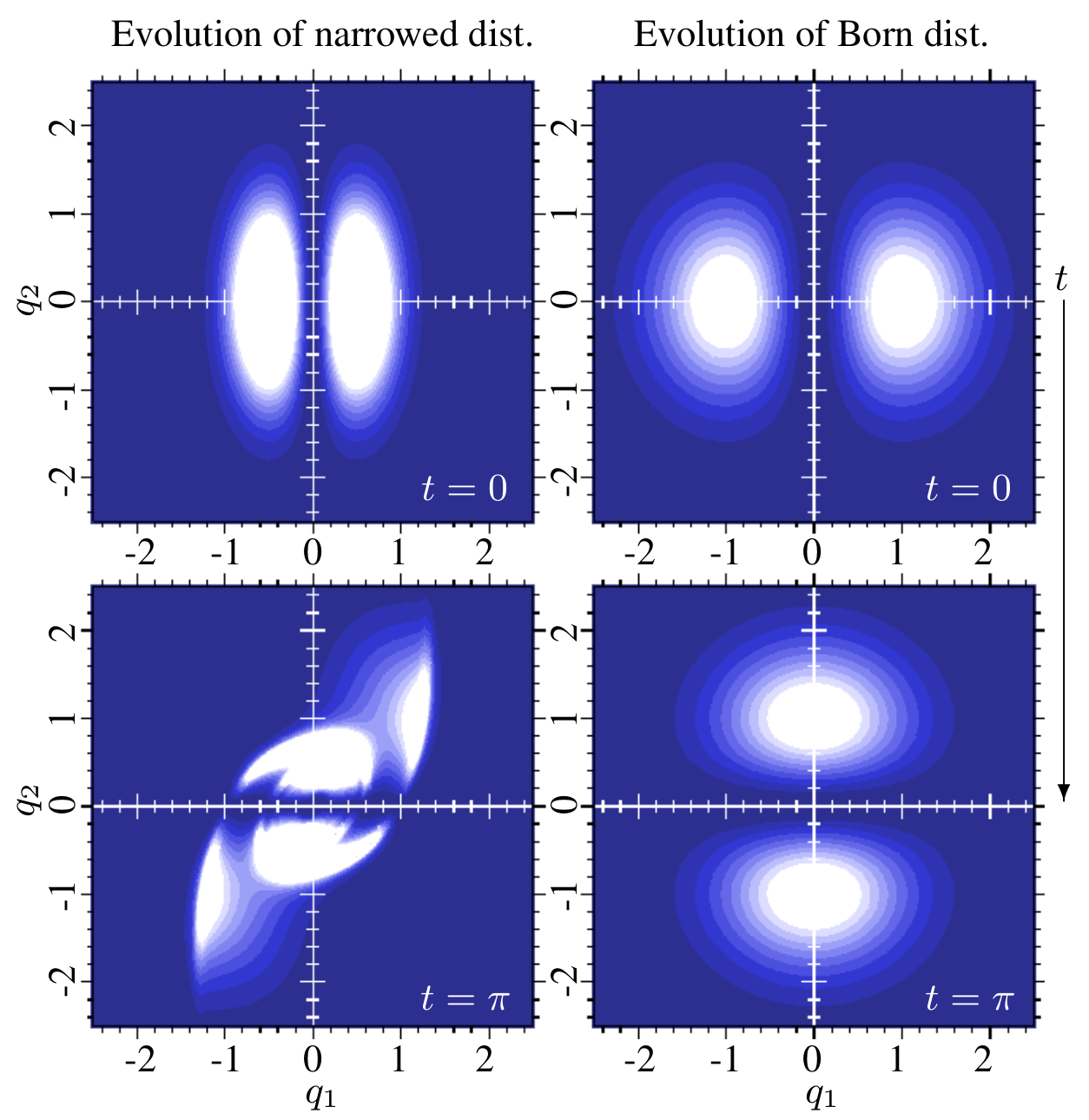
How does Liouville's theorem cause relaxation?
Dark colored regions indicate large \(\rho(q,p)\).
Light colored regions small \(\rho(q,p\)).
Remember:
- The entropy is a measure of how spread out the distribution is.
- But Liouville's theorem (information conservation) prevents the distribution spreading or changing color.
This is a phase space diagram depicting density of \(\rho(q,p,t)\) for the Hamiltonian
$$H=\frac{1}{2}p^2+q^4-q^3-q^2-q.$$
How does Liouville's theorem cause relaxation?
It stirs the states around subject to an perfectly incompressible, liquid-like flow.
The resulting distribution ends up looking something like cotton-wool or scrunched-up newspaper.
Eventually the structure becomes too fine to detect in reasonable experiment:
1) Imagine detecting that shape from individual point sources with a telescope.
2) Imagine the sample size you would need.
3) Imagine the resolution required.
How does Liouville's theorem cause relaxation? (continued)
If the previous slide was the 'wordy' version of the justification, the mathematical version is the H-theorem.
H-theorem inputs:
- Liouville's theorem
- Assumption of no fine-tuning
- Coarse-graining (or discretization, or pixelation or rasterization).
H-theorem outputs:
- Entropy rise (relaxation)
| Ingredient | |
|---|---|
| 1) State-space | |
| 2) Law of evolution | |
| 3) Equilibrium distribution | |
| 4) Information measure | |
| 5) Information conservation | |
| 6) De facto entropy rise |
\Omega = \mathbb{R}^n
S=-\int_\Omega \rho\log\rho\, \mathrm{d}^nx
Uniform
Continuous iRelax theories
(Based upon differential entropy)
H-theorem
Now all ingredients have been found for the differential entropy case except the law of evolution
Liouville's theorem
| Ingredient | |
|---|---|
| 1) State-space | |
| 2) Law of evolution | |
| 3) Equilibrium distribution | |
| 4) Information measure | |
| 5) Information conservation | |
| 6) De facto entropy rise | H-theorem |
\Omega = \mathbb{R}^n
S=-\int_\Omega \rho\log\rho\, \mathrm{d}^nx
Uniform
Continuous iRelax theories
(Based upon differential entropy)
Constraints on the law of motion
As noted earlier, entropy conservation restricts laws to be incompressible,
$$\sum_i\frac{\partial \dot{x}_i}{\partial x_i}=\nabla.\dot{x}=0.$$
Take for instance a simple two dimensional state space \(x=(q,p)\in \mathbb{R}^2\). Then the velocity may be Helmholtz decomposed as
$$\dot{x}=\underbrace{\nabla A}_{=0} + \left( \begin{matrix} 0&-1\\1&0\end{matrix}\right)\nabla B.$$
So the equation of motion is necessarily
$$\dot{q} = -\frac{\partial B}{\partial p},\quad\quad\dot{p}=\frac{\partial B}{\partial q},$$
for some scalar function \(B(q,p)\).
Classical mechanics (Hamilton's equations) are obtained in the case that \(B=-H\).
\nabla.\dot{x}=0
Liouville's theorem
There is not enough time for:
-
A discussion on the arrow of time
-
The development of 'suitable' coordinates and 'suitable' transforms.
-
An explanation of how these ideas work in classical field theories.
The emergence of time asymmetry from an explicitly time symmetric theory.
Like canonical transforms. Useful.
Generally expect equations that are supposed to describe fundamental behavior to conserve entropy. In the thesis this is shown explicitly for the Klein-Gordon field. Equations that only describe effective behavior would generally not be expected to conserve information, and this is shown explicitly for the heat equation.
Generalize by correcting for the problems with differential entropy.....
S=-\int_\Omega \rho\log\rho\, \mathrm{d}^nx
Dimensionally inconsistent due to logarithm of dimensionful quantity.
In contrast to discrete Gibbs entropy, which is invariant under relabelings of states, \(i\rightarrow j(i)\), differential entropy is expected to change under relabelings, \(x\rightarrow y(x)\).
This point is fleshed out in the section on suitable coordinates.
There is an ambiguity in extending the principle of indifference to continuous states.
The natural extension of "equal probabilities" to a continuous space is the "uniform" probability distribution.
But as many coordinate choices are possible, the question soon arises as to which set of coordinates the distribution should be uniform in.
(cf. Bertrand's paradox.)
Appears not to be derived (by Shannon), but merely written down.
These problems are corrected for through the use of the Jaynes entropy
Introduce the Jaynes Entropy
S=-\int_\Omega \rho\log\rho\, \mathrm{d}^nx
Consider deriving a continuous entropy by generalizing the Gibbs entropy.
$$\underset{\bullet}{x_{i-4}}\quad \underset{\bullet}{x_{i-3}}\quad \underset{\bullet}{x_{i-2}}\quad \underset{\bullet}{x_{i-1}}\quad \underset{\bullet}{x_i} \quad \underset{\bullet}{x_{i+1}}\quad \underset{\bullet}{x_{i+2}}\quad \underset{\bullet}{x_{i+3}}\quad \underset{\bullet}{x_{i+4}}$$
Associate discrete states with a continuous position
Take the limit as these become dense

$$m(x)$$
$$x$$
Cannot assume uniform limit, so density of states \(m(x)\) is introduced.
S=-\int_\Omega \rho\log\frac{\rho}{m}\, \mathrm{d}^nx
Differential entropy
Jaynes Entropy
How do the iRelax ingredients change?
S=-\int_\Omega \rho\log\frac{\rho}{m}\, \mathrm{d}^nx
| Ingredient | Differential entropy | Jaynes Entropy |
|---|---|---|
| 1) State-space | ||
| 2) Law of evolution | ||
| 3) Equilibrium distribution | Uniform | m(x) |
| 4) Information measure | Liouville's theorem | Modified L'theorem |
| 5) Information conservation | ||
| 6) De facto entropy rise | H-theorem | Valentini's theorem |
\Omega = \mathbb{R}^n
S=-\int_\Omega \rho\log\rho\, \mathrm{d}^nx
\nabla.\dot{x}=0
\Omega = \mathbb{R}^n
Ingredient 3:
- The equilibrium distribution must now be uniform w.r.t. the density of states \(m(x)\).
- But \(m(x)\) and \(\rho_\text{eq}(x)\) are both normalized, so $$\rho_\text{eq}(x)=m(x).$$
d\rho/dt=0
Ingredient 4:
The Green's function/propagator formalism may be used to derive a modified Liouville theorem,
$$\begin{matrix} 1) & \frac{d\rho}{dt}=0\rightarrow \frac{d}{dt}\left(\frac{\rho}{m}\right)=0 \\ 2) & |\det\mathbf{J}(x_i\to x_f)|=1\rightarrow |\det\mathbf{J}(x_i\to x_f)|=\frac{m(x')}{m(x)}\\3)& \nabla\cdot\dot{x}=0\rightarrow \nabla\cdot(m\dot{x})=0 \end{matrix}$$
\nabla\cdot(m\dot{x})=0
d(\rho/m)/dt=0
Relaxation in quantum physics?
Corollary 1:
The Born distribution is a density of states.
$$m(x)= |\psi(x,t)|^2$$
Central Motivation:
Regard quantum probabilities as equilibrium probabilities.
$$m(x) = |\psi(x,t)|^2$$
Corollary 3:
Conservation of information/entropy
$$\frac{d}{dt}\left(\frac{\rho}{m}\right)=0 \longrightarrow \frac{d}{dt}\left(\frac{\rho}{|\psi|^2}\right)=0$$
| Ingredient | |
|---|---|
| 1) State-space | |
| 2) Law of evolution | |
| 3) Equilibrium distribution | |
| 4) Information measure | |
| 5) Information conservation | Modified L'theorem |
| 6) De facto entropy rise | Valentini's theorem |
\Omega = \mathbb{R}^n
De facto entropy rise:
Still Valentini's theorem
|\psi(x,t)|^2
S=-\int_\Omega \rho\log\frac{\rho}{|\psi|^2}
d/dt(\rho/|\psi|^2)=0
Corallary 2: $$ \begin{matrix} \text{Jaynes Entropy}\\ S=-\int_\Omega \rho\log\frac{\rho}{m}\, \mathrm{d}^nx \\ \downarrow \\ \text{Valentini Entropy}\\ S=-\int_\Omega \rho\log\frac{\rho}{|\psi|^2}\, \mathrm{d}^nx \end{matrix}$$
Relaxation in quantum physics?
Law of evolution:
The constraint placed on the law of evolution is modified to
$$\nabla\cdot j(x,t)=-\frac{\partial |\psi(x,t)|^2}{\partial t}.$$
If a solution \(j(x,t)\) is that satisfies this equation, then the law of evolution,
$$\dot{x}=\frac{j(x,t)}{|\psi(x,t)|^2},$$
will relax to an equilibrium \(\rho_\text{eq}=|\psi|^2\).
Once one solution is found , others follow by adding an incompressible current, \({\nabla.j_\text{inc}(x,t)=0}\), so that
$$\dot{x}'=\dot{x}+\frac{j_\text{inc}}{|\psi|^2}.$$
Canonical de Broglie-Bohm solution:
For point particles:
$$\dot{q}_i =\frac{\hbar}{m_i}\text{Im}\left(\frac{\partial_{q_i} \psi}{\psi}\right)\quad\text{or}\quad \dot{q}_i = \frac{\partial_{q_i} S}{m_i},$$
where \(\psi(q_1,q_2,...)=|\psi(q_1,q_2,...)|e^{iS(q_1,q_2,...)/\hbar}\).
For a bosonic field:
$$\dot{\phi}(y)\sim\text{Im}\left(\frac{1}{\psi}\frac{\delta\psi}{\delta\phi(y)}\right)\quad \text{or}\quad \dot{\phi}(y)\sim\frac{\delta S}{\delta\phi(y)},$$
where \(\psi[\phi]=|\psi[\phi]|\exp(iS[\phi])\).
Non-canonical solution by Green's functions:
In an arbitrary basis \( \left. | x \right>\), for \(x\in\mathbb{R}^n\),
$$\dot{x}\sim\frac{1}{|\psi(x)|^2} \int_\Omega\mathrm{d}^nx' \frac{\widehat{\Delta x}}{|\Delta x|^{n-1}} \frac{\partial |\psi(x')|^2}{\partial t}.$$
Relaxation in action in de Broglie-Bohm theory
Suggested observations to make:
- Observe the vorticies. These surround the nodes of the wave function, and produce a good deal of 'mixing'.
- Observe the fine structure forming and becoming ever finer until it is imperceptible with the sample size.
- Look for artifacts of incomplete relaxation.
An imperfect fit?
True iRelax theories map states to other states as:
\dot{x}:\mathbb{R}^n\longrightarrow\mathbb{R}^n
x:\mathbb{R}^n\times\mathbb{R}\longrightarrow\mathbb{R}^n
x\longmapsto \dot{x}(x)
(x_0,t)\longmapsto x(x_0,t)
\dot{x}:\mathbb{R}^n\times\mathcal{H}\longrightarrow\mathbb{R}^n
x:\mathbb{R}^n\times\mathbb{R}\times\mathcal{H}\longrightarrow\mathbb{R}^n
(x,\psi)\longmapsto \dot{x}(x,\psi)
(x_0,t,\psi)\longmapsto x(x_0,t,\psi)
Whereas de Broglie-Bohm type theories map states to other states as:
So it becomes interesting to speculate whether quantum theory will admit a complete iRelax framework that unifies de Broglie-Bohm with canonical quantum theory.
Open questions about quantum relaxation
(The remainder of this talk will consider only de Broglie-Bohm theory.)
Chapter 2 of the thesis (Part 2 of this talk) describes how systems tend to relax toward equilibrium, but it does not say whether quantum equilibrium will actually be reached. Is it reasonable to expect relaxation to conclude quickly for all (non-trivial) systems?
In classical systems there exist barriers to quantum relaxation. Do there exist similar barriers to quantum relaxation?
If a distribution is very out-of-equilibrium, how does this affect relaxation time?
Energy states freeze relaxation trivially. Are there other quantum states for which relaxation is frozen or impeded?
How can a single composite system mimic equilibrium in its sub-systems?
How does relaxation speed depend upon the dimensionality of the system in question?
Recent papers discussing these topics:
Abraham, Colin, Valentini, Long-time relaxation in pilot-wave theory, J. Phys, A, 47 2014
A. Kandhadai and A. Valentini. Perturbations and quantum relaxation. Found. Phys., 49, 2019
Chapter 3 - What is it?
A study of quantum relaxation in the context of the isotropic 2-dimensional oscillator (equivalent to an uncoupled field mode) with quite a lot of small results...
\frac{1}{2}\left(\partial_\eta^2+\eta^{-1}\partial_\eta+\eta^{-2}\partial_\varphi^2+\eta^2\right)\psi=i\overset{\circ}{\psi}
\overset{\circ}{\eta}=\text{Im}(\partial_\eta\psi/\psi),\quad\overset{\circ}{\varphi}=\eta^{-2}\text{Im}(\partial_\varphi\psi/\psi)
One of the distinguishing features is the use of dual bases
\frac{1}{2}\left(\partial_{Q_x}^2+\partial_{Q_y}^2+Q_x^2+Q_y^2\right)\psi=i\overset{\circ}{\psi},
Angular
Cartesian
\overset{\circ}{Q_x}=\text{Im}(\partial_{Q_x}\psi/\psi),\quad\overset{\circ}{Q_y}=\text{Im}(\partial_{Q_y}\psi/\psi)
a_d^\dagger=\frac{1}{\sqrt{2}}\left(a_x^\dagger + ia_y^\dagger\right),\quad a_g^\dagger=\frac{1}{\sqrt{2}}\left(a_x^\dagger-ia_y^\dagger\right)
\psi=\sum_{n_d n_g}C_{n_d n_g}e^{-i(n_d+n_g)T}\chi_{n_d n_g}
\psi=\sum_{n_n n_y}D_{n_x n_y}e^{-i(n_x+n_y)T}\psi_{n_x n_y}
The following is a list of properties of nodes.
(i) Nodes are points.
This follows trivially as \(\psi=0\) places two real conditions on the two-dimensional space.
(ii) The velocity field has zero vorticity away from nodes.
Velocity is \(\sim\nabla S\), so \(\nabla\times v=0\) everywhere except on nodes, where \(S\) is ill-defined.
(iii) The vorticity of nodes is 'quantised'.
As a consequence of the above results,
$$\oint_{\partial \Sigma}v.\mathrm{d}l=\oint_{\partial \Sigma}\mathrm{d}S=2\pi n,$$for integer \(n\), and where \(\partial\Sigma\) is a simple closed loop.
Nodal properties subject to an energy limit and no fine-tuning
(iv) Nodes generate chaos.
From the \(v\sim 1/r\) dependence.
(v) Nodes pair create/annihilate.
Condition \(\psi=0\) defines two plane algebraic curves, with nodes appearing upon the intersections of these lines.
(vi) Vorticity is locally conserved.
Consider the line integral of \(v\) around a pair creation/annihilation event.
(vii) Nodes have \(\pm2\pi\) vorticity.
A result of complex-ifying one of the dimensions and computing the loop integrals as contour integrals. (No fine-tuning.)
(viii) Vorticity is globally conserved.
A result of boundedness of energy, found with the angular basis.
(ix) States of total vorticity \(V_\text{tot}\) have a minimum of \(V_\text{tot}/2\pi\) nodes.
This follows from properties (vii) and (viii). Of course, pair creation allows there to be more than this number.
(x) The ‘vorticity theorem’ provides a simple method by which the total vorticity of a state may be calculated.
Calculate the conserved quantity \(V_\text{tot}\) from the quantum state parameters. Uses the argument principle of complex analysis.
(xi) A state that is bounded in energy by \(n_d+n_g=m\) may only take the following \(m+1\) possible total vorticities
$$\mathcal{V}_\text{tot}=-2\pi m,\; -2\pi m+4\pi,\;\dots,\\ \dots \;2\pi m-4\pi,\;2\pi m.$$
Follows from the vorticity theorem. Clean categories of states.
(xii) A state that is bounded in energy by \(n_d+n_g=m\) has a maximum of \(m^2\) nodes.
The condition of a node may be written as the intersection of two plane algebraic curves of degree \(m\). By Bézout's theorem (originally found in Newton's Pricipia), the most that this can happen is \(m^2\) times.
So for example...
\mathcal{V}_\text{tot}=-2\pi m,\; -2\pi m+4\pi,\; \dots \;2\pi m-4\pi,\;2\pi m
Min nodes \(=\mathcal{V}_\text{tot}/2\pi\)
Max nodes \(=m^2\)
Can use the vorticity theorem to calculate which of these the quantum state is.
\(m=1\)
\(\mathcal{V}_\text{tot}=-2\pi\quad\text{or}\quad 2\pi\)
MIN 1 node
MAX 1 node
MIN 1 node
MAX 1 node
\(m=2\)
\(\mathcal{V}_\text{tot}=-4\pi\quad\text{or}\quad 0\quad\text{or}\quad 4\pi\)
MIN 2 nodes
MAX 4 nodes
MIN 0 nodes
MAX 4 node
MIN 2 nodes
MAX 4 nodes
\(m=3\)
\(\mathcal{V}_\text{tot}=-6\pi\quad\text{or}\quad -2\pi\quad\text{or}\quad 2\pi\quad\text{or}\quad 6\pi\)
MIN 3 nodes
MAX 9 nodes
MIN 1 node
MAX 9 nodes
MIN 1 node
MAX 9 nodes
MIN 3 nodes
MAX 9 nodes
\(m=4\)
\(\mathcal{V}_\text{tot}=-8\pi\quad\text{or}\quad -4\pi\quad\text{or}\quad 0\pi\quad\text{or}\quad 4\pi\quad\text{or}\quad 8\pi\)
MIN 4 nodes
MAX 16 nodes
MIN 2 nodes
MAX 16 nodes
MIN 0 nodes
MAX 16 nodes
MIN 2 nodes
MAX 16 nodes
MIN 4 nodes
MAX 16 nodes
Extreme quantum nonequilibrium

The "bulk" of the Born distribution, containing "most" nodal activity and chaotic trajectories.
The "tails" of the Born distribution, containing "little" nodal activity and regular trajectories.
For the purposes of this chapter, extreme quantum nonequilibrium is defined to be that in which the distribution is appreciably separated from the bulk of the Born distribution.

Extreme quantum nonequilibrium
Roughly divide the relaxation timescale into 2 parts:
$$t_\text{total relaxation time}\sim t_\text{reach bulk}+t_\text{efficient relaxation}$$
But,
$$t_\text{reach bulk}\gg t_\text{efficient relaxation}.$$
So,
$$t_\text{total relaxation time}\sim t_\text{reach bulk}.$$
So \(t_\text{reach bulk}\) is of primary concern.
Drift fields
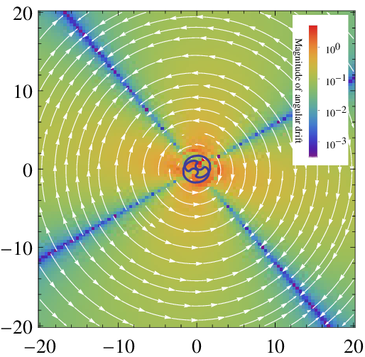
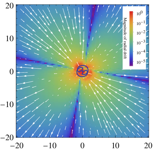
- For a grid of initial positions, evolve trajectories with high precision through a single wave function period using a standard numerical method.
- Record the final displacement vector from the original position for each grid point.
- Plot the grid of displacement vectors as a vector field. (It is useful to plot the radial and angular components separately, as the angular component will often be significantly larger.)
The basic method:
The resulting drift field may be regarded as a time-independent velocity field of sorts, and used to track long-term evolution without the need for large computational resources as would usually be the case.
(I made several thousand of these for the referee.)
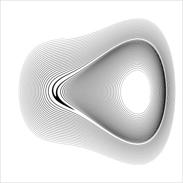
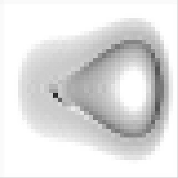
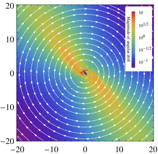
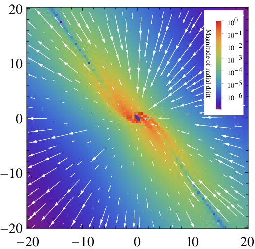
Drift fields Type-0
In the states studied (up to \(M=15\)), drift fields fell into 3 distinct categories, namely type-0, type-1, and type-2.
Angular Part
Radial Part
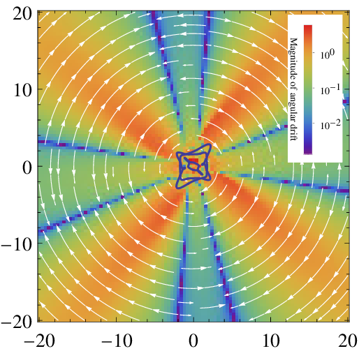
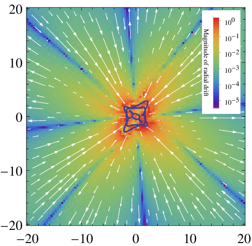
Drift fields Type-1
Angular Part
Radial Part
In the states studied (up to \(M=15\)), drift fields fell into 3 distinct categories, namely type-0, type-1, and type-2.
Drift fields Type-2
Angular Part
Radial Part
In the states studied (up to \(M=15\)), drift fields fell into 3 distinct categories, namely type-0, type-1, and type-2.
Angular Part
Radial Part
Type-1 and type-2 drift fields feature a clear mechanism to transport trajectories to the center, hence causing relaxation of extreme nonequilibrium
Type-0 drift fields have a conspicuous absence of any parallel relaxation mechanism, and appear to inhibit or perhaps even prevent transport to the center. For these quantum states, quantum relaxation is in the least retarded and may be prevented altogether.
The referee didn't believe me so I made them this figure.


Radial displacement after 1000 trajectories
The quantum states used were those that produced the type-0 and type-1 drift fields on the earlier page.
The vorticity drift conjectures
After a survey of many procedurally generated quantum states (and noting their relative frequency) I decided to zoom in on two conjectures. I ran a much more targeted study of two groups of quantum states. The result is the following. Their truth is argued mainly on the basis of lack of counter-example.
Conjecture 1 - A state with zero total vorticity cannot produce a type-0 drift field.
Two thousand procedurally generated \(\mathcal{V}_\text{tot}=0\) states checked (by hand).
Conjecture 2 - All states of maximal vorticity produce type-0 drift fields.
Four thousand procedurally generated \(\mathcal{V}_\text{tot}=\mathcal{V}_\text{max}\) states checked (by hand).
(Useful as provides a means to calculate the relaxation inhibiting states for further study.)
Alternative title:
Antony and I consider relic nonequilibrium in particles from two angles.
Investigation 1
Investigation 2
The matter available to the majority of common experiment has a long and violent astrophysical history.
It is not unreasonable therefore to expect any initial quantum nonequilibrium to have long since decayed away.
We asked the question:
Is it possible that there exist systems (particles) for which quantum nonequilibrium may have been preserved?
Predicting whether or not quantum nonequilibrium could persist is difficult.
It depends on uncertain factors -
- Beyond the standard model particle physics
- Early Universe (pre-hot big bang) cosmology
- Quantum relaxation in many-body systems and on cosmological scales
Of the matter we know to exist, there is one prime candidate for a nonequilibrium carrier, namely dark matter.
We asked the question:
If dark matter exhibited quantum nonequilibrium, how might this show up in experiment?
Investigation 1
Is it possible that there exist systems (particles) for which quantum nonequilibrium may have been preserved?
First illustrative scenario: Inflaton decay
\(t_\text{Planck}\)
\(t\)
Inflation
Preheating
Reheating
Pre-Inflationary radiation dominated era
Planck Era
Particle creation by inflaton decay.
Particle creation by parametric resonance. Due to the kinetic energy of the 'classical part' of inflaton field.
Post-Inflation
\varphi(\mathbf{x},t)=\phi_{0}(t)+\phi(\mathbf{x},t)
Super-Hubble field modes experience retarded relaxation (\(t_\text{ret} (t)\ll t )\). So may reasonably expect to find nonequilibrium at sufficiently large wavelengths.
(This is the source of Antony's long-wavelength CMB power deficit stuff.)
Relaxation does not take place at all during inflation. This comes from a treatment of the Bunch-Davies vacuum.
"Trans-Planckian" modes may transfer exotic gravitational effects. (Has been argued that quantum nonequilibrium is gravitationally unstable.)
Nonequilibrium in inflaton passed on to created particles.
Nonequilibrium in fermionic vacuum retained after particles created.

First illustrative scenario


\gamma
DM particle
DM particle in quantum nonequilibrium
Annihilation (or decay)
nonequilibrium photon
Telescope
\gamma
DM particle
DM particle in quantum nonequilibrium
Annihilation (or decay)
nonequilibrium photon
First illustrative scenario
Telescope
To avoid subsequent relaxation, and be detectable the nonequilibrium DM particles would need to satisfy the following two criteria.
1) Particles must be created at a time after their corresponding decoupling time \(t_{\mathrm{dec}}\) (when the mean free time \(t_{\operatorname{col}}\) between collisions is larger than the expansion timescale \(t_{\exp}\equiv a/\dot{a}\)) or equivalently at a temperature below their decoupling temperature \(T_{\mathrm{dec}}\). Otherwise the interactions with other particles are likely to cause rapid relaxation.
2) In order for them to be detectable they must decay or annihilate into photons. But in order for these photons to avoid relaxation, this would need to occur after \((t_\text{dec})_\gamma\).
A natural candidate to consider is the gravitino, \(\tilde G\). A simple estimate suggest a restriction to gravitinos produced at temperatures \(\lesssim 10^{-7}T_P\).
Second illustrative scenario
Vacuum modes are energy eigenstates, and so trivially avoid relaxation. Is it possible that some vacuum modes could live through the early Universe without getting excited?
For a given field there are 3 mechanisms that can cause excitations:
(i) Inflaton decay
(ii) Interactions with other fields
(iii) Spatial expansion
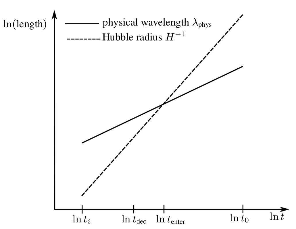
While a field mode is in the super-Hubble regime, it will be shielded from the effects of local physics.
If, during the post-inflationary radiation-dominated phase the mode enters the Hubble radius at time \(t_\text{enter}\) that is greater than the fields decoupling time \(t_\text{dec}\), it will remain unexcited.
Excitation by spatial expansion does not occur for conformally coupled fields.
Only possible for massless fields: photon, massless neutrino, gravitino
\mathcal{L}=\frac{1}{2}\sqrt{-\,g}\left( \,g_{\mu\nu}\partial^{\mu}%
\phi\partial^{\nu}\phi-\frac{1}{6}\,R\phi^{2}\right)
To support our arguments:
Vacuum modes are energy eigenstates, and so trivially avoid relaxation. Is it possible that some vacuum modes could live through the early Universe without getting excited?
We built a model of two coupled fields in a box and showed that quantum nonequilibrium passes from one to the other:
We modeled simple von Neumann measurements to build a model of two coupled fields in a box and showed that quantum nonequilibrium passes from one to the other:
Investigation 2
If dark matter exhibited quantum nonequilibrium, how might this show up in experiment?
Return to the original scenario
\gamma
DM particle
DM particle in quantum nonequilibrium
Annihilation (or decay)
nonequilibrium photon
Telescope
A reliable estimate of relaxation seems difficult, as it depends upon the aforesaid unknown factors. Instead consider what may be said about this end of the scenario.
We focused on the search for "smoking gun" line spectra, which has had a lively and controversial last few years.
Why are our effects interesting?
\rho_\text{obs}(E)=\int D(E|E_\gamma)\rho_\text{true}(E_\gamma)\mathrm{d}E_\gamma.

D(E|E_\gamma)
\rho_\text{true}(E_\gamma)
The telescope energy dispersion.
Due to the interaction of the telescope with the photon.
The true profile.
Most of the shape due to Doppler broadening. (See refs. in thesis).
A line spectrum recorded in one of the single-photon-detection telescopes envisaged interacts with each photon, ultimately producing an observed spectrum according to:
\rho_\text{obs}(E)=\int D(E|E_\gamma)\rho_\text{true}(E_\gamma)\mathrm{d}E_\gamma.
D(E|E_\gamma)
\rho_\text{true}(E_\gamma)


Regime 1 of 2: The high resolution telescope
Narrow
Wide
The telescope energy dispersion.
Due to the interaction of the telescope with the photon.
The true profile.
Most of the shape due to Doppler broadening. (See refs. in thesis).
\rho_\text{obs}(E)=\int D(E|E_\gamma)\rho_\text{true}(E_\gamma)\mathrm{d}E_\gamma.
D(E|E_\gamma)
\rho_\text{true}(E_\gamma)
Regime 1 of 2: The high resolution telescope
Narrow
Wide
\rho_\text{obs}(E)\approx \rho_\text{true}(E)
The high resolution telescope may resolve the profile of the spectral line.
The telescope energy dispersion.
Due to the interaction of the telescope with the photon.
The true profile.
Most of the shape due to Doppler broadening. (See refs. in thesis).
\rho_\text{obs}(E)=\int D(E|E_\gamma)\rho_\text{true}(E_\gamma)\mathrm{d}E_\gamma.
D(E|E_\gamma)
\rho_\text{true}(E_\gamma)
Regime 2 of 2: The low resolution telescope
Narrow
Wide
\rho_\text{obs}(E)\approx D(E|E_\text{true})
The low resolution telescope instead observes its own energy dispersion.
Most telescopes used for line searches are in this regime.
The telescope energy dispersion.
Due to the interaction of the telescope with the photon.
The true profile.
Most of the shape due to Doppler broadening. (See refs. in thesis).
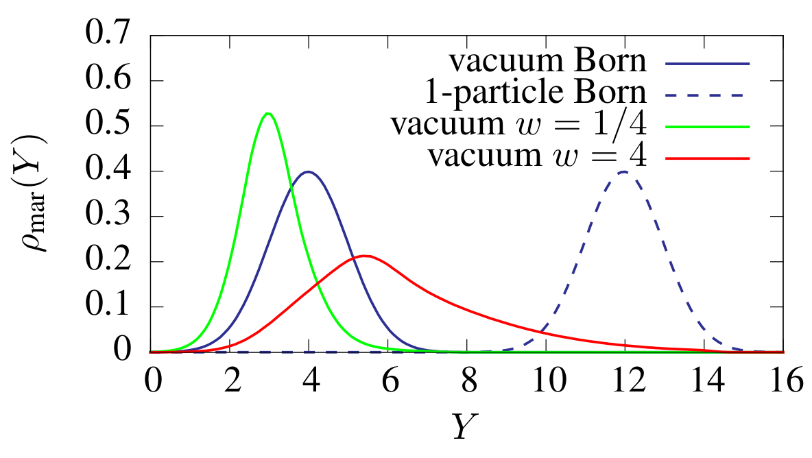
A simple model of photon spectral measurement
\frac{\Delta E}{E}\sim \frac{1}{T}
Key point: As the model progresses, in effect it describes the outcome of an increasingly high resolution telescope:
This is the measurement of an equilibrium ensemble of photons
A simple model of photon spectral measurement
Key point: As the model progresses, in effect it describes the outcome of an increasingly high resolution telescope:
A nonequilibrium ensemble
\frac{\Delta E}{E}\sim \frac{1}{T}
A simple model of photon spectral measurement
Key point: As the model progresses, in effect it describes the outcome of an increasingly high resolution telescope:
Another nonequilibrium ensemble
\frac{\Delta E}{E}\sim \frac{1}{T}
Further Reading:
Relic quantum nonequilibrium
N. G. Underwood and A. Valentini. Quantum field theory of relic nonequilibrium systems.
Phys. Rev. D, 92, 2015, arXiv:1409.6817.
N. G. Underwood and A. Valentini. Anomalous spectral lines and relic quantum nonequilibrium. 2016, arXiv:1609.04576 (submitted to Phys. Rev. D)
Nodes, drift fields, relaxation retarding states and all that
Nicolas G. Underwood. Extreme quantum nonequilibrium, nodes, vorticity, drift and relax-
ation retarding states. J. Phys. A. 51, 2018, arXiv:1705.06757
The iRelax framework
This thesis only.
A universalist view of Bell's theorem
In preparation.
Thank you for listening.
Nicolas G. Underwood PhD Defense
By Nick Underwood
Nicolas G. Underwood PhD Defense
Signatures of Relic Quantum Nonequilibrium


