Part 1:

What is Ergodicity?

Physicists

Ergodic theory

Mathematicians

Economists, Medics, and social scientists

Dynamical Behaviour

Statistical Laws

A much debated correspondence

Two Contentious Arguments

1. The Ergodic Hypothesis
2. The H-Theorem

• Statistical mechanics is a study of the statistical/probabilistic laws that arise out of dynamical systems.
• But the hows, the whens, the wherefores, and the under what circumstances(es) of how these statistical laws arise has been a point of contention since the birth of the discipline. 
• It is where this question is borderline, that some of the more interesting, exotic behaviour occurs. 

The subject of this new project and of this seminar

Central to another project I have ongoing and of the next seminar

Boltzmann's Ergodic Hypothesis

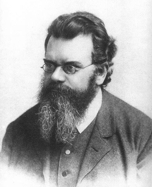
• The term Ergodic was introduced in an 1884 paper by Boltzmann [cite]
• Appears to have taken earlier inspiration from Helmholtz who noted that monocyclic systems could provide a basis for thermodynamical laws.
• From the beginning it appears to be only loosely defined, and exactly what Boltzmann meant is has been the source of debate.
• One statement of the alleged property:

If let run for an infinite time, a single trajectory constrained on a constant energy surface would fill the entirety of the available phase space.

$$\begin{matrix}\text{The infinite time average of function f}\\\text{ over a single trajectory}\end{matrix}=:\hat{f}\,\,=\,\,\bar{f}:=\begin{matrix}\text{The equilibrium ensemble}\\\text{ average of function f}\end{matrix}$$

Consequently: 

Establishes:

1. The very use of probability theory and statistical explanations in physics
2. The uniqueness of the invariant phase probability density used in statistical mechanics
3. The unimportance of the initial dynamical state.

Boltzmann appears to have held a "resolutely finitist" view of the energy surface, viewing it as divisible into a countable number of cells, which would be visited equally by a single trajectory.

and also:

The independence of the time average on initial conditions.

Selected notions of ergodicity

• Ludwig Boltzmann (1884)
  Original ergodic hypothesis
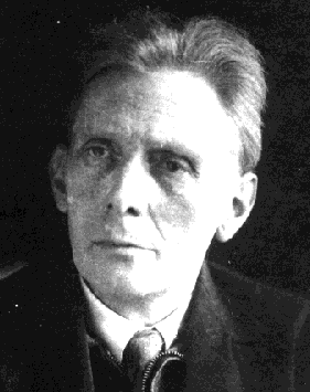
• George David Birkhoff (1931)
  I) Existence of infinite time average,
  II) Metric Transitivity (MT) \(\implies\) ergodicity
• John Von Neumann (1932)
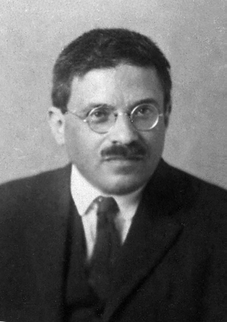
  Mean Ergodic Theorem - Holds on Hilbert spaces, subject to certain conditions we won't go into here
• Aleksandr Khinchin (1949)
  Self similarity argument (SSA)
• Paul and Tatiana Ehrenfest (1956)
  Quasi-Ergodic Hypothesis - "Almost all" initial points result in a trajectory that densely covers the phase space
• Contemporary pragmatic definition

Birkhoff

von Neumann

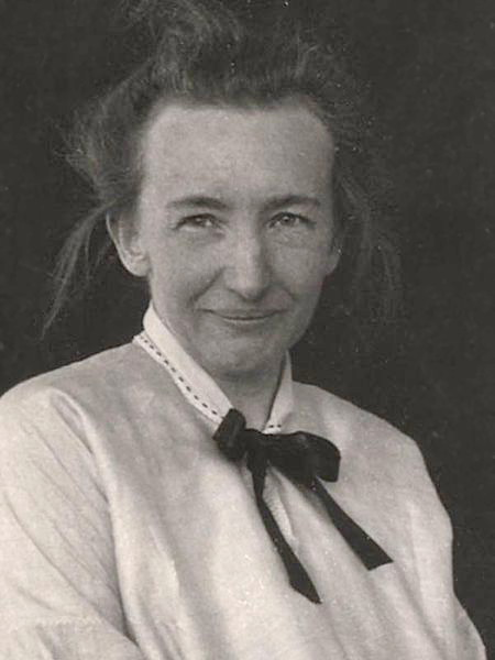
Tatyana
Afanasyeva

Paul Ehrenfest

Khinchin

Boltzmann

Ergodicity regarded as a property of the dynamics resulting in \(\hat{f}=\bar{f}\)

A rough sketch of how the notion of ergodicity changed over time

Certain functions can be ergodic, and others not so. Ergodicity is then a property of both the dynamics and the function being averaged. The test of ergodicity is whether \(\hat{f}=\bar{f}\)

The property that \(\hat{f}=\bar{f}\) became the accepted, pragmatic definition of ergodicity, rather than its consequence

Selected notions of ergodicity

• Ludwig Boltzmann (1884)
  Original ergodic hypothesis
• George David Birkhoff (1931)
  I) Existence of infinite time average,
  II) Metric Transitivity (MT) \(\implies\) ergodicity
• John Von Neumann (1932)
  Mean Ergodic Theorem - Holds on Hilbert spaces, subject to certain conditions we won't go into here
• Aleksandr Khinchin (1949)
  Self similarity argument (SSA)
• Paul and Tatiana Ehrenfest (1956)
  Quasi-Ergodic Hypothesis - "Almost all" initial points result in a trajectory that densely covers the phase space
• Contemporary pragmatic definition

Birkhoff

von Neumann

Tatyana
Afanasyeva

Paul Ehrenfest

Khinchin

Boltzmann

Here we will first cover Metric Transitivity as it helps to introduce some of the formal mathematical background of the subject. We'll then touch on Khinchin's Self-Similarity argument so as to contrast the quite stark difference of its formulation, before moving on to our proposed (much more operational) approach to the question of ergodicity.

Background

Probability space

We begin with a Kolmogorov style probability space, the tuple

$$(\Omega, \sigma, \mu),$$

where

• \(\Omega = \) the sample space (physicists read state/phase space),
• \(\sigma = \) the sigma algebra - in short, all the subsets of the sample space that could correspond to meaningful statements. For instance, the roll of the die is greater than 4, or the momentum of particle \(i\) is positive, or the center of mass is equal to some value,
• \(\mu = \) the measure of the space. 

A probability space is a measure space in which the measure of the whole space is unity, \(\mu(\Omega)=1\).

Measure preserving dynamics

We add to the probability space a measure preserving dynamics \(T\), 

$$(\Omega, \sigma, \mu, T).$$

The measure is preserved by the dynamics in the sense that for all \(\omega\in \sigma \),

$$\mu(T(\omega)) = \mu(\omega).$$

Although it is possible to consider other circumstances (more discussion on this as we go), following on from its origins in classical mechanics, ergodic theory as a discipline is usually introduced in terms of a measure preserving dynamics.

So we'll start there:

The measure maps elements of the \(\sigma\) onto probabilities,

$$\mu: \sigma \rightarrow [0,1],$$

so that if \(\Omega\) is spanned by coords \(x\in\Omega\), and \(\omega\) is a member of the sigma algebra, \(\omega\in\sigma\), then

$$ \mu: \omega \mapsto \mu(\omega)=\int_\omega d\mu =\int_\omega \mu(x)dx=\begin{matrix}\text{proportional of}\\ \text{total states in }\omega\end{matrix} \in [0,1]$$

In simple terms, \(\mu(x)=\) the density of states at coordinates \(x\).

Understanding the measure

• The measure translates regions of the space \(\omega\), with dimensions of \(\left[x\right]\) into probability, which can be understood to be equal to proportion of total states inside the region. Thought of as a density,
  $$\mu(x)= \frac{\text{proportion of states}}{\text{volume}}.$$
• Probably the most familiar measure to physicists is the Liouville measure from classical mechanics, which corresponds to a uniform \(\mu(x)\); simply the volume of the region as measured in canonical coordinates,
  $$\mu(\omega)=\text{Vol}(\omega).$$
• The requirement that the measure is preserved is then simply the classical Liouville theorem,
  $$\text{Vol}(T(\omega)) = \text{Vol}(\omega).$$

How physicists tend to think of the measure

Reasons to account for a non-uniform measure

• More exotic types of dynamics do exist inside and outside of physics.
• Even if the underlying dynamics is classical, we may be tracing over some of the degrees of freedom, and so only considering an effective theory. (cf. BBGKY hierarchy?)
• Ultimately, the generalization of the principle of indifference to continuous spaces is problematic. (cf. Bertrand's paradox)
• Even discrete models may violate the principle of indifference. (cf. weighted dice)

We already have seen that the measure of any volume is conserved by the dynamics

$$\mu(T(\omega)) = \mu(\omega).$$
 

Definition (Invariant Volume)

An invariant volume \(\omega_\text{inv}\) is a region of the state space that is unchanged by the dynamics
$$T(\omega_\text{inv}) = \omega_\text{inv}$$

The whole space is an invariant volume
The path followed by a single trajectory is an invariant volume (albeit of measure zero)
 

Definition (Metrically Indecomposable Invariant Volume)

A metrically indecomposable (MI) volume, \(\omega_\text{MI}\), is a invariant volume that cannot be decomposed into two smaller invariant volumes
$$\omega_\text{MI}\neq \omega_\text{1,inv}+\omega_\text{2,inv}$$

Metric Transitivity I

A very crudely sketched out invariant volume 

In this case the volume is not MI, as we could divide into smaller invariant volumes

Metric Transitivity II

Theorem (Birkhoff I)

The time average of a function over a trajectory exists in in the long time limit,

$$\hat{f}(x) := \lim_{t\rightarrow\infty} \frac{1}{t} \int_0^t f(T(x,t'))dt'$$

exists "almost everywhere" in \(\Omega\). (We'll state this without proof.)

Note: this means we should regard infinite time averages as functions of entire trajectories.

Lemma

The infinite time average  \(\hat{f}(x)\) is constant almost everywhere on an MI volume, \(\omega_\text{inv}\).

Proof

• Suppose there exists \(x_1\) and \(x_2\) such that
  $$\hat{f}(x_1)< \hat{f}(x_2).$$  ​
• Pick some value \(\alpha\) between these two values,
  $$\hat{f}(x_1) <\alpha <\hat{f}(x_2)$$
• Divide \(\omega_\text{inv}\) up into two regions, one for which \(\hat{f}(x)<\alpha \,\forall \,x\), and one in which \(\hat{f}(x)\geq \alpha \,\forall\, x\).
• These are invariant volumes in their own right, and so we have reached a contradiction. \(\blacksquare\)

We already have seen that the measure of any volume is conserved by the dynamics

$$\mu(T(\omega)) = \mu(\omega).$$
 

Definition (Invariant Volume)

An invariant volume \(\omega_\text{inv}\) is a region of the state space that is unchanged by the dynamics
$$T(\omega_\text{inv}) = \omega_\text{inv}$$

The whole space is an invariant volume
The path followed by a single trajectory is an invariant volume (albeit of measure zero)
 

Definition (Metrically Indecomposable Invariant Volume)

A metrically indecomposable (MI) volume, \(\omega_\text{MI}\), is a invariant volume that cannot be decomposed into two smaller invariant volumes
$$\omega_\text{MI}\neq \omega_\text{1,inv}+\omega_\text{2,inv}$$

Definition - Metric Transitivity (MT)

A system for which almost the entire space \(\Omega\) is metrically indecomposable is called Metrically Transitive (MT).

Theorem (Birkhoff II - Metric Transitivity)

A system which is MT satisfies

$$\hat{f}(x)=\bar{f}(x)$$

for almost all states \(x\in\Omega\).

Metric Transitivity III

Proof

• Introduce a finite time average
  $$\hat{f}_c(x)=\frac{1}{c}\int_0^c f(x)dt.$$
• When the ensemble average of this is taken, it essentially overrides the temporal average
  $$\overline{\hat{f}_c(x)} = \frac{1}{\mu(\Omega)} \int_\Omega \hat{f}_c(x) d\mu = \frac{1}{c \mu(\Omega)} \int_\Omega \int_0^c f(x)dt d\mu = \frac{\bar{f}(x)}{c}\int_0^cdt = \bar{f}(x), $$
  assuming we can switch the order of integration.
• Now consider the difference between \(\hat{f}(x)\) and \(\bar{f}(x)\),
  $$\hat{f}(x) - \bar{f}(x) = \frac{1}{\mu(\Omega)} \int \left\{ \hat{f}(x)- \hat{f}_c(x)\right\} d\mu$$
• The above quantity is not dependent upon time parameter \(c\), and in the limit \(c\rightarrow\infty\), we have \(\hat{f}_c(x)= \hat{f}(x)\). Hence the right side vanishes, and must do for all \(c\). Hence \(\hat{f}(x)=\bar{f}(x).\quad \blacksquare \)

Are real systems Metrically Transitive I?

MT is a rigorous notion of ergodicity, very much in the spirit of Boltzmann, and which guarantees \(\hat{f}=\bar{f}\). So are familiar systems MT?

Is the simple Hamiltonian system I've been using as an example MT?

No..... Trajectories follow paths upon closed surfaces of constant energy. Any interval between two energies is an invariant volume, and these may be divided ad nauseam, so not MT.

 What if we considered only systems of a given energy?

Well..... Restricting to a microcanonical (MC) ensemble, with implied measure \(\mu_\text{MC}\), would indeed make this particular system MT.

However....

\(E_1\)

\(E_2\)

Are real systems Metrically Transitive II?

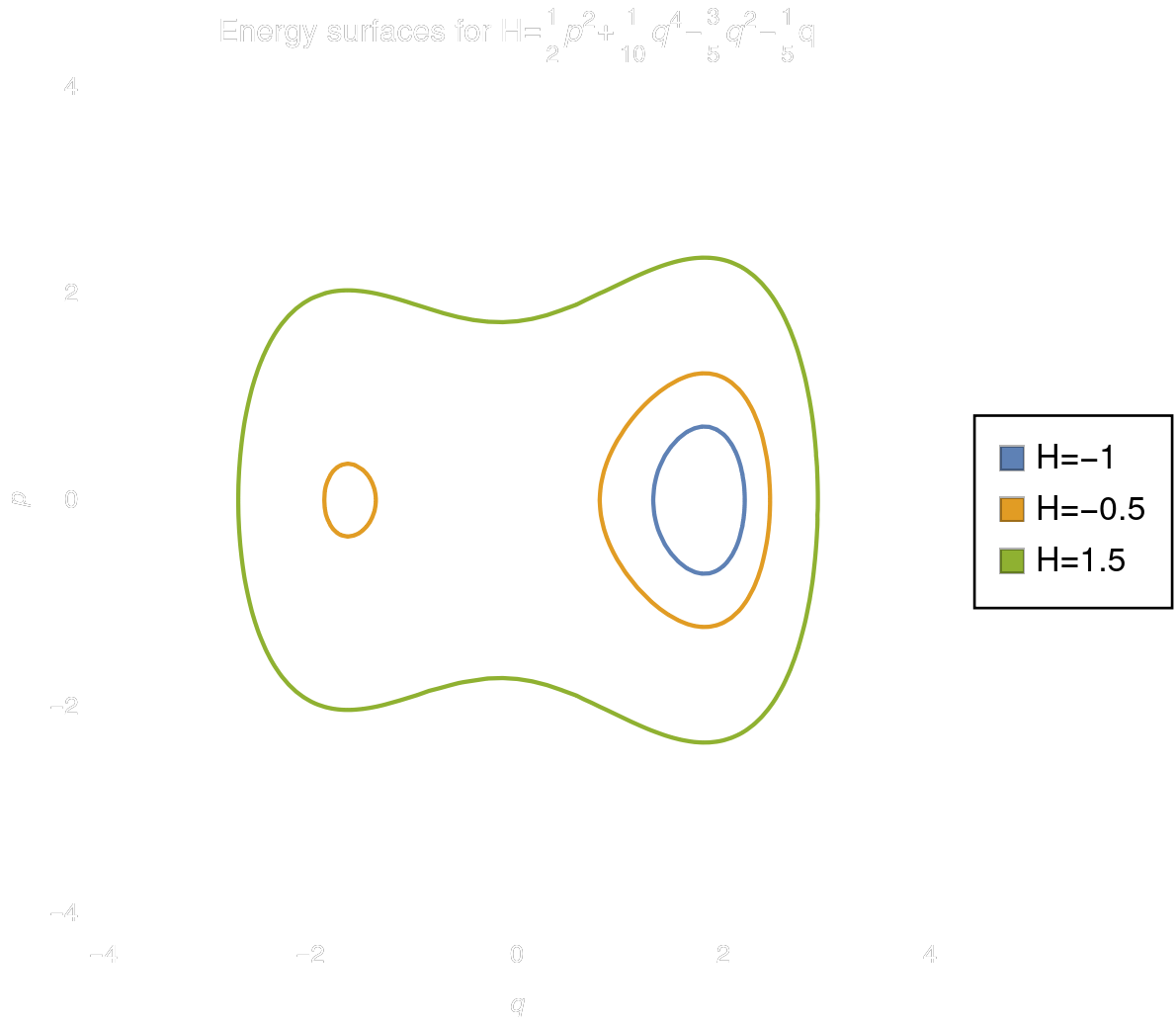
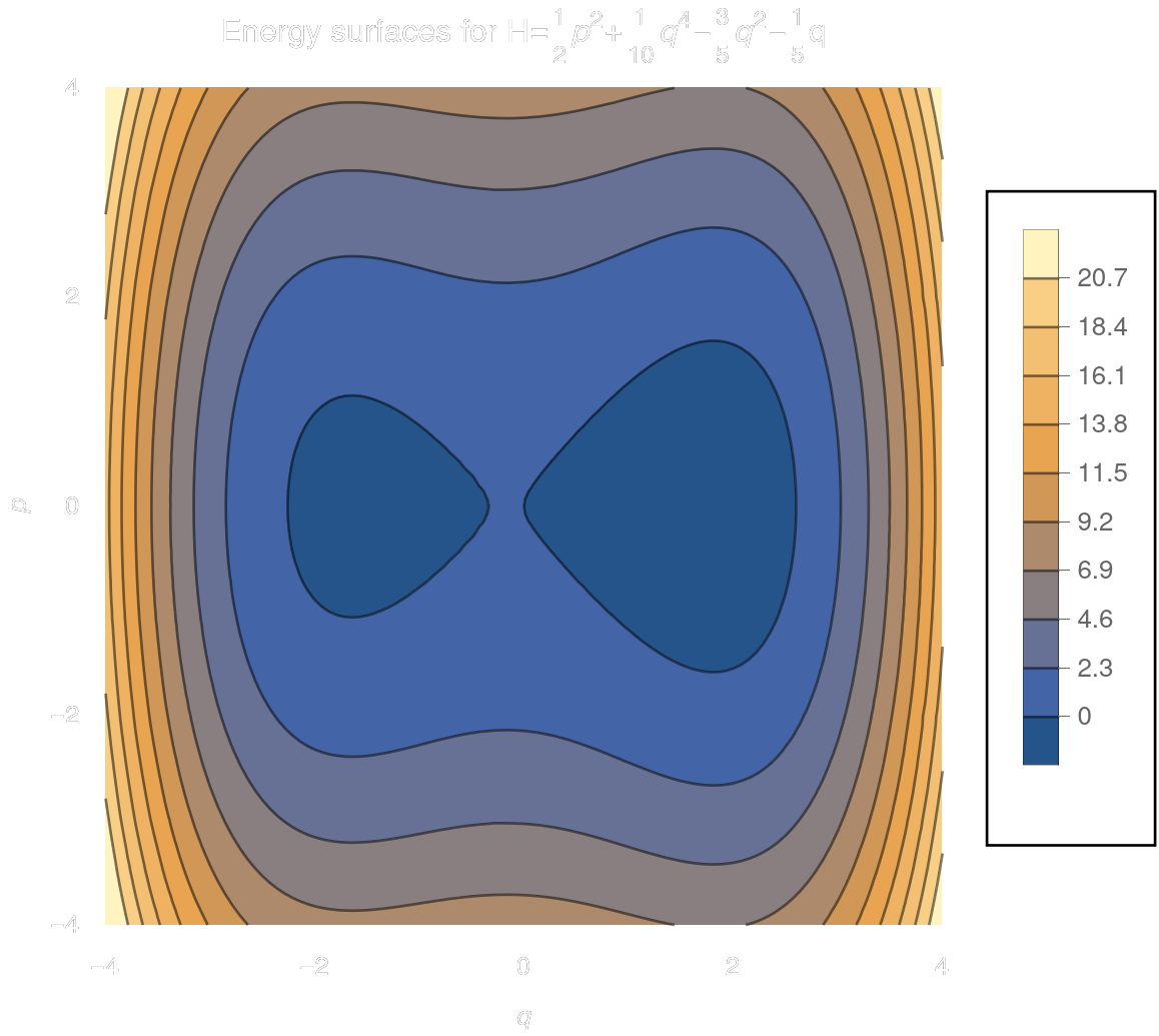
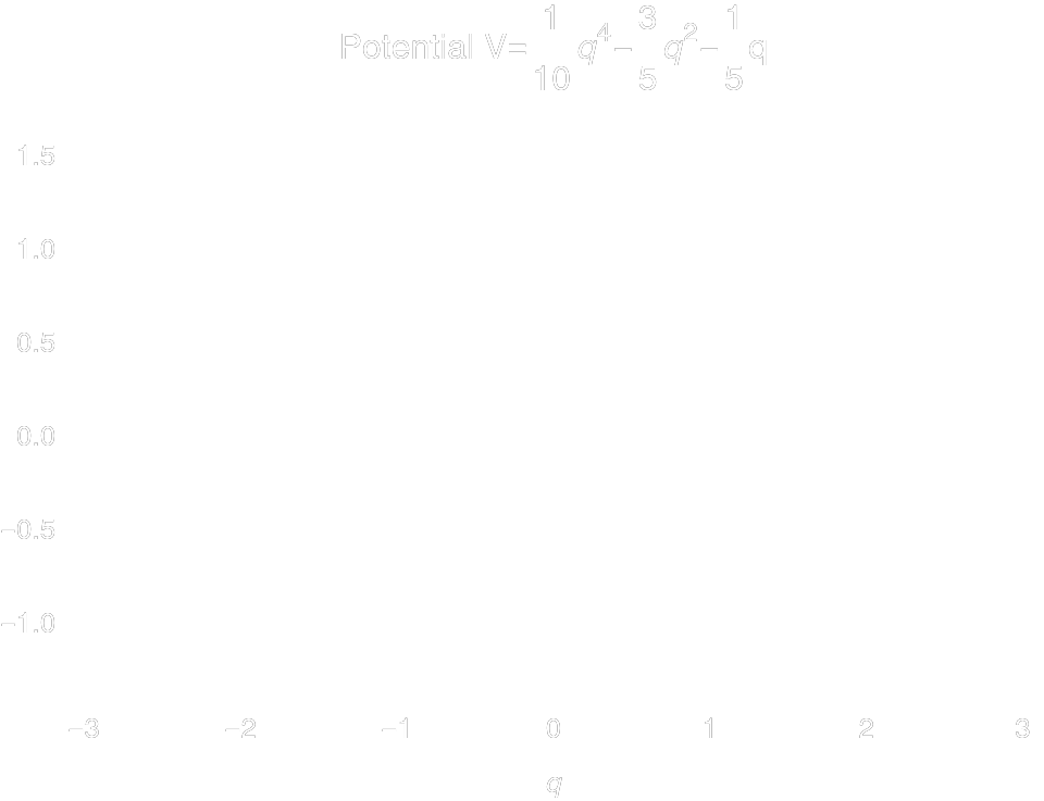
...Even the smallest change to the potential breaks this in an interesting/complicated way.

The chief qualitative difference between this system and the last is that I have slightly modified the potential to add this local minimum here.

This changes the energy surfaces so that between \(\sim -0.6 \) and \(\sim 0.0\) they become disconnected.

Above these energies MT \(=\checkmark\)

Below these energies MT \(=\checkmark\)

Between the energies MT \(=\times\)

(....and clearly \(\hat{f}\neq\bar{f}\) for an arbitrary \(f\).)

Ergodicity without Metric Transitivity?

• Aside from very simple model systems such as hard spheres in a box, it is very hard to demonstrate MI for remotely realistic systems with non-singular interactions.
• While MT is mathematically well defined, Khinchin noted that it was unnecessarily too strong a condition to justify the use of the ergodic hypothesis for most applications in physics.
• Khinchin instead proposed a system based upon generic statistical considerations. The result is his Self

Aleksander Khinchin

1. A separable Hamiltonian
   $$H=\sum_{n}^NH_n(q_n,p_n)$$
2. Only special additive "sum functions" considered,
   $$f=\sum_{n}^Nf_n(q_n,p_n)$$
3. Number of particles must be large, $$N\gg1$$
4. Regions of small but finite measure exist in which \(\hat{f}\neq\bar{f}\) (at least for finite \(N\)).

Resulting Inequality

$$\text{Prob}\left(\frac{|\hat{f}-\bar{f}|}{|\bar{f}|}\geq K_1 N^{-1/4}\right)\leq K_2N^{-1/4},$$
where \(K_1\) and \(K_2\) are \(O(1)\). In short, as a system grows larger, the probability of finding a deviation from ergodicity beyond a certain size shrinks, vanishing in the thermodynamical limit.

Assumptions of Khinchin's scheme:

Interactions would break this condition. Khinchin argued that a physical Hamiltonian need only be approximately seperable.

For instance kinetic energy, or pressure, but suffers similar conceptual problem with interaction potentials.

The need for a more practical approach

Requires an infinite time

(no experiment is run for an infinite time)

Khinchin's Self-Similarity Argument

Birkhoff's Metric Transitivity

Only applies to very large systems - many interesting systems are relatively small

May apply (with difficulty) to short range interactions, but doesn't apply to long range interactions

Only applies to specific additive functions

Aside from simple model systems (e.g. hard spheres in a box) very difficult to assess/prove for realistic systems with non-singular interactions

Doesn't allow us to assess or measure lack of ergodicity (meaning \(\hat{f}\neq\bar{f}\)), or prove it's absence 

• Both of these methods provide certain conditions under which \(\hat{f}\neq\bar{f}\) holds.
• But they are not the only way of assessing whether \(\hat{f}\neq\bar{f}\).
• Ideally we'd have a general method, applicable to all dynamical systems, that assesses ergodicity for finite times and for finite system sizes, and that provides a measure of ergodicity, not simply a way of proving it's presence or ruling it out.

Part 2:

Our proposed approach

...or, how can we add to this picture?

Outline of the problem in practical terms

Defining a practical notion of ergodicity

The commonly held notion of ergodicity is simply the equality of the two averages,

$$\hat{f}:=\lim_{t\rightarrow\infty}\int_0^t f\left(T(x,t)\right)\mathrm{d}t,\quad \quad \bar{f}:=\frac{1}{\mu(\Omega)}\int_\Omega f \mathrm{d}\mu$$

• In practical experimental or computational circumstances, we cannot know \(\bar{f}\) and  \(\hat{f}\). We must sample them.
• So, out of our code we extract two lists of numbers,
  $$f_t:=\{f_t^{(1)},f_t^{(2)},...,f_t^{(n)}\}\quad\quad\text{and}\quad\quad f_e=\{f_e^{(1)},f_e^{(2)},...,f_e^{(n)}\}.$$
• Intuitively, ergodicity is the tendency of a single trajectory to traverse the space in such a way that it samples the same underlying distribution as the ensemble.
  
  
  
  
   
• We define a system to be Ideally Ergodic (IE) if \(f_t\) and \(f_e\) are two finite realisations of the same underlying distribution.

Assessing Ideal Ergodicity I

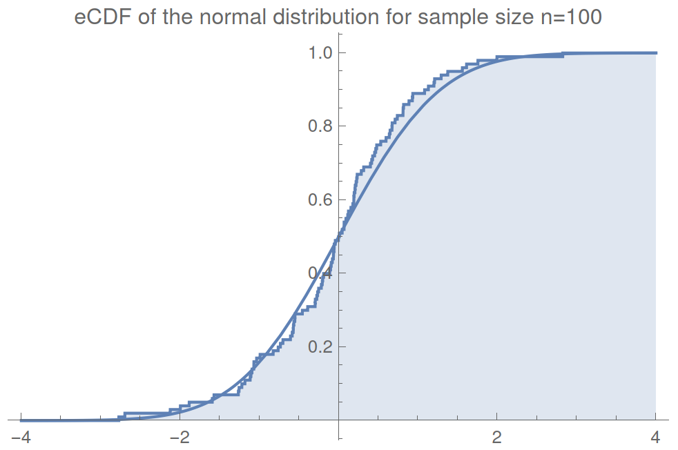
Empirical cumulative distribution functions (eCDFs)

We can translate samples \(f_t\) and \(f_e\) into eCDFs, 

$$F^n_t(f_t):=\frac{1}{n}\sum_i^n\Theta(f^{(i)}_t), \quad F^n_e(f_e):=\frac{1}{n}\sum_i^n\Theta(f^{(i)}_e),$$

where \(\Theta\) is the Heaviside step function.
For example - Here is a randomly sampled normal distribution:

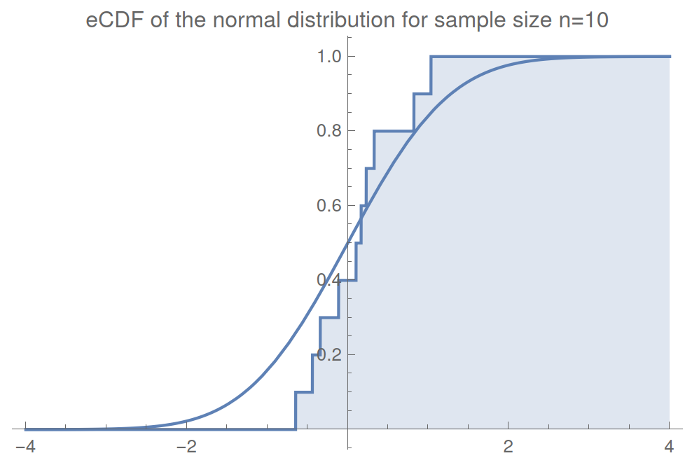
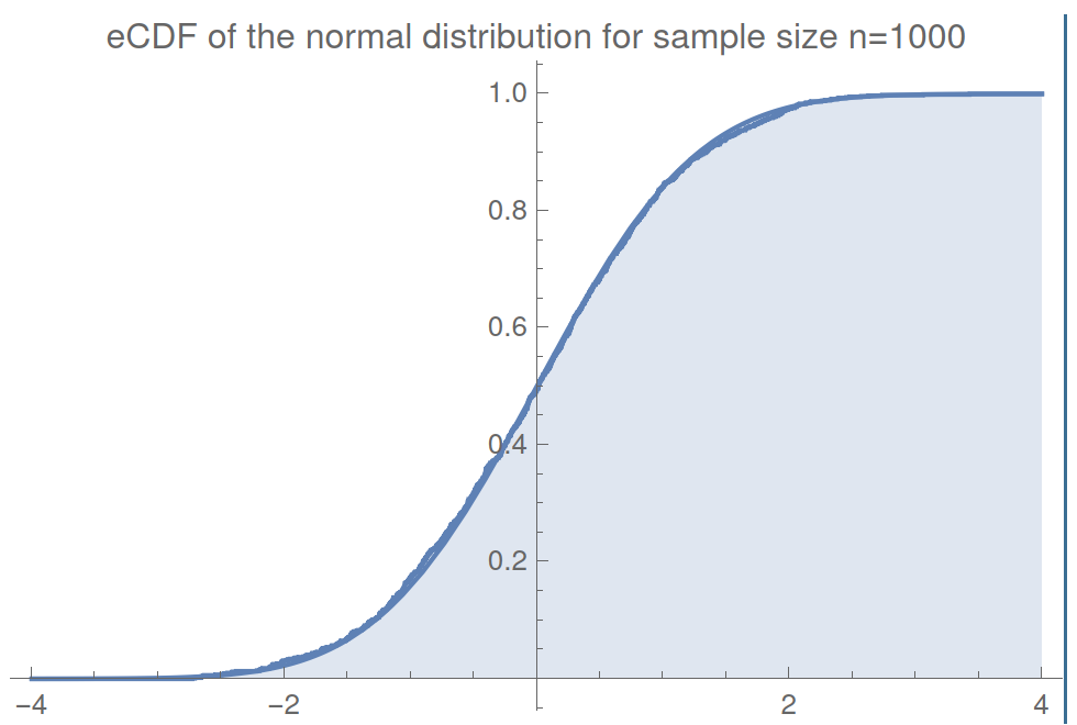
eCDFs make fiinite jumps of \(1/n\) at each value in the sample.

Assessing Ideal Ergodicity II

Empirical cumulative distribution functions (eCDFs)

We can translate samples \(f_t\) and \(f_e\) into eCDFs,

$$F^n_t(f_t):=\frac{1}{n}\sum_i^n\Theta(f^{(i)}_t), \quad F^n_e(f_e):=\frac{1}{n}\sum_i^n\Theta(f^{(i)}_e),$$

where \(\Theta\) is the Heaviside step function.

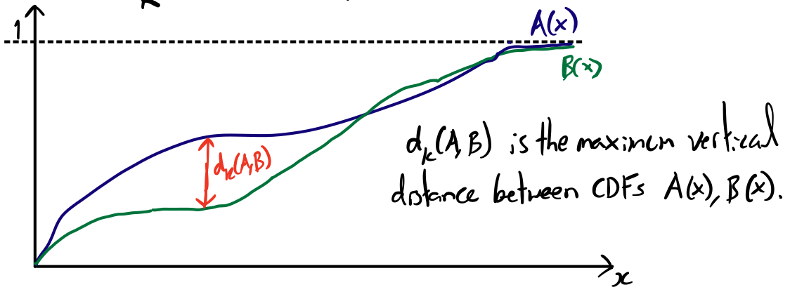
Assessing the similarity of two distributions
To assess the difference between two distributions can use the Kolmogorov-Smirnov (KS) metric,
$$d_K(A,B):=\text{sup}_x\left|A(x)-B(x)\right|,$$
which is the maximum "vertical" distance between distributions.

For eCDFs of equal sample size \(n\) the KS metric takes quantised values \(d_K=m/n\) for integer \(m\) between 0 and n.

This makes KS distances of eCDFs very quick to assess computationally.

Assessing Ideal Ergodicity III

Convergence of \(d_K(F^n_t,F^n_e)\)

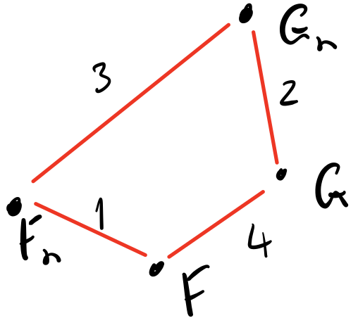
• Since the KS metric is indeed "metric", it obeys a triangle inequality

$$d_K(A,C)\leq d_k(A,B)+d_K(B,C)$$

• We can make use of this by considering triangle inequalities involving both sampled distributions \(F^n_t,F^n_e\), and underlying distributions \(F_t,F_e\). It follows that
  $$|d_K(F^n_t,F^n_e)-d_K(F_t,F_e)|\leq d_K(F^n_t,F_t)+ d_K(F^n_e,F_e).$$
• The Glivenko-Cantelli theorem determines the asymptotic behaviour of sampled eCDFs,
  $$d_K(F^n,F)\rightarrow 0$$ almost surely in the limit as \(n\rightarrow\infty\).
• Hence \(\,d_K(F^n_t,F^n_e)\rightarrow d_K(F_t,F_e)\) almost surely in the limit \(n\rightarrow\infty\). (\(d_K(F_t,F_e)=0\) was the definition of ideal ergodicity.)

What is it possible to say about about \(d_K(F_t,F_e)\)?
While it isn't possible to know \(d_K(F_t,F_e)\) from finite samples, we can still try inquire about it, for instance by,

1. Assume \(d_K(F_t,F_e)=0\) and seek incompatibility with sampled data.
2. ​Seek reasonable upper bounds, or another way of quantifying lack of ergodicity.

Hypothesis testing ideal ergodicity I

Uniform distribution

Normal distribution

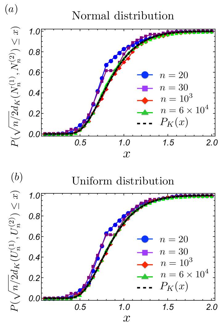
Kolmogorov-Smirnov distribution

• Suppose that two underlying distributions are known to be equal, \(A=B\), so that \(d_K(A,B)=0\).
• Then the KS distance calculated from the corrresponding sampled distributions, \(d_K(A^n,B^n)\), is known to obey the KS (cumulative) probability distribution,
  $$\text{CDF}(x)=\frac{\sqrt{2\pi}}{x}\sum_{k=1}^{\infty}e^{-\frac{(2k-1)^2\pi^2}{8x^2}}$$

Remarkably, this is true regardless of the underlying distribution!
This allows us to hypothesis test using IE as the null hypothesis.

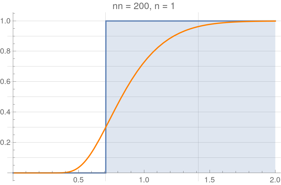
A figure made by Fabien showing convergence to the KS distribution with increasing \(n\)

The equivalent figures made by me with a Mathematica code

Hypothesis testing ideal ergodicity II

Standard hypothesis testing algorithm

1. Let \(F_t=F_e\) be the null hypothesis and \(F_t\neq F_e\) be the alternative hypothesis.
2. For a given value of \(n\), the null hypothesis implies finding a sampled distance beyond a certain value
   $$d_K(F^n_e,F^n_t)> K^{(2)}_n(\alpha)$$ has a probability of less than \(\alpha\).
3. If \(\alpha\) is sufficiently small, say 0.01, then such an observation is deemed sufficiently unlikely to reject the null hypothesis.  

Kolmogorov-Smirnov distribution

• Suppose that two underlying distributions are known to be equal, \(A=B\), so that \(d_K(A,B)=0\).
• Then the KS distance calculated from the corrresponding sampled distributions, \(d_K(A^n,B^n)\), is known to obey the KS (cumulative) probability distribution,
  $$\text{CDF}(x)=\frac{\sqrt{2\pi}}{x}\sum_{k=1}^{\infty}e^{-\frac{(2k-1)^2\pi^2}{8x^2}}$$

Remarkably, this is true regardless of the underlying distribution!
This allows us to hypothesis test using IE as the null hypothesis.

• Such a test was used to reject IE for some amplitudes of a tapped granular system in Paillusson and Frenkel Phys. Rev. Lett. 109, 208001 (2012).

• However, as it is formulated, this test does not permit to make any clear proposition regarding how much ergodic a function f is.

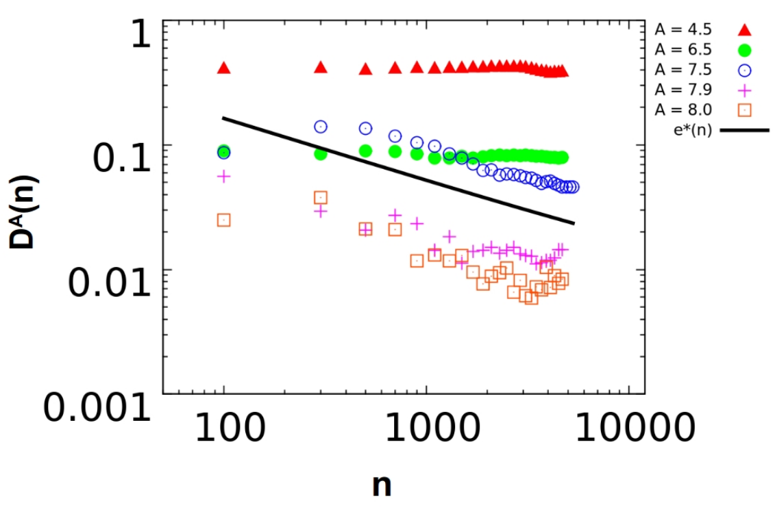
A plot from that paper.

Another Example

Another figure I've borrowed from Fabien:
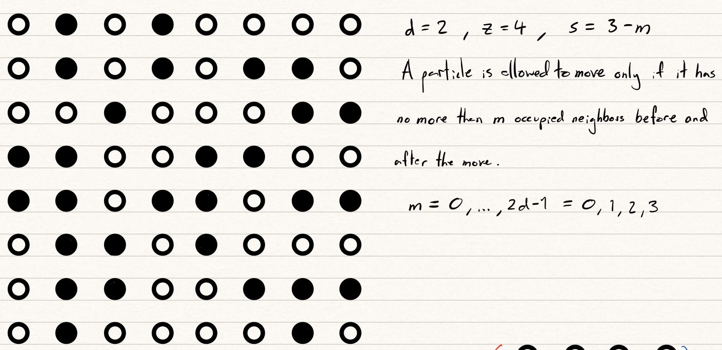
Preliminary analysis of the mean contact number on a \(10\times 10\) lattice at different densities.

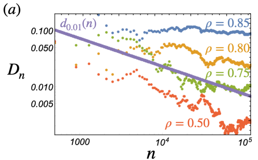
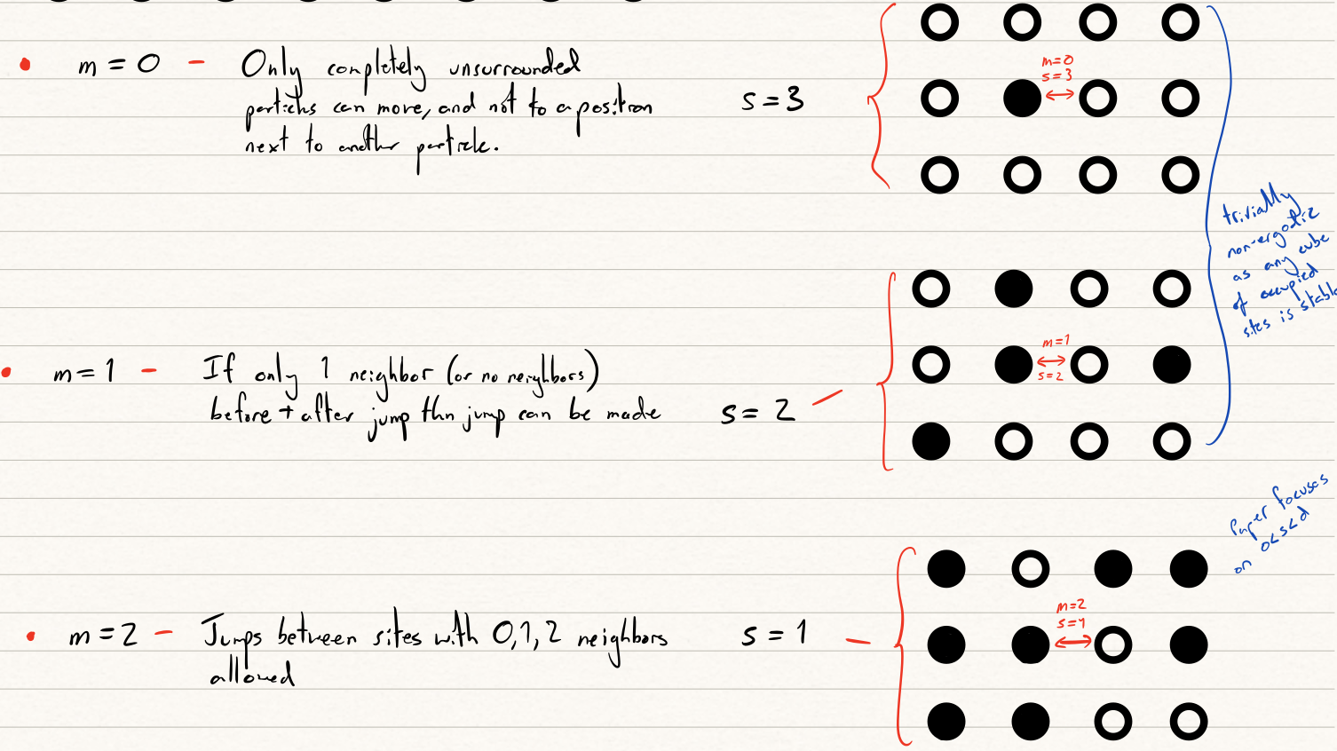
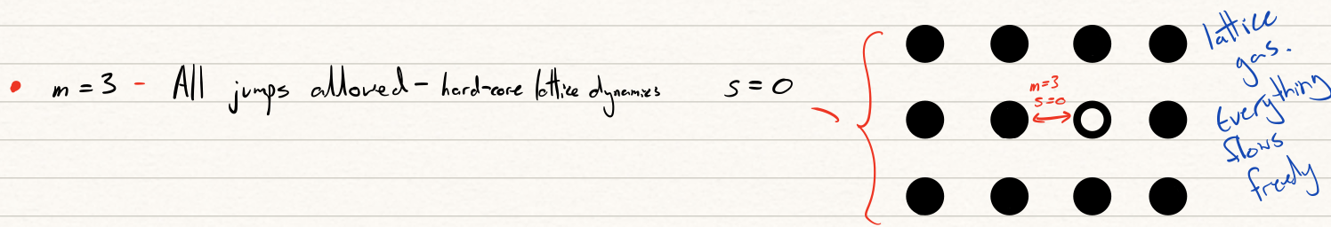
The Kob-Anderson model is a discrete lattice model introduced to study glassy phase transitions through ergodicity. A particle is permitted to jump between sites on if it has no more than \(m\) occupied neighbours before and after the move.

Going further with fuzzy logic

(Note: You may have to forgive me here. At this point it is not just the logic, but my understanding that becomes fuzzy...)

It may be wasteful to simply reject a hypothesis of ergodicity once a somewhat arbitrary cut-off point has been reached. The system in question may still be approximately ergodic and approximate statistical mechanics may follow. Instead we might think to tailor a new definition of ergodicity based upon fuzzy logic. 

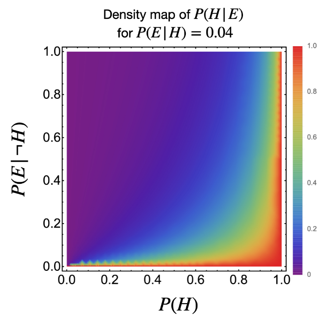
Fuzzy logic applied to Statistical Hypothesis Testing
The familiar law of Modus Tollens (contraposition) from classical logic says that

$$\text{If  }A\implies B\text{    then    } \lnot B\implies \lnot A$$
In the context of hypothesis testing, the uncertainties involved means this does not carry directly over,

$$P(E|H)<0.01 \neq P(\lnot H| E)>99\%$$
Matt Booth and Fabien have a paper published earlier this year on how Fuzzy logic may be used to address this issue.

A figure from Booth, Paillusson, A Fuzzy Take on the Logical Issues of Statistical Hypothesis Testing. Philosophies 2021, 6, 21.

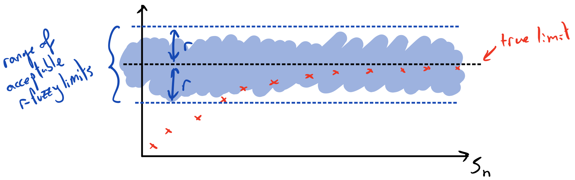
\(r\)-fuzzy limits
$$\underset{n\rightarrow\infty}{\text{Fuzlim}}S_n=a \text{  iff  }\forall \epsilon>0\,\,\exists n>n_\epsilon \text{  s.t.  } |S_n-a|\leq r+\epsilon$$ 

\(r\)-fuzzy convergence
A sequence \(s(t)\) is called \(r\)-fuzzy convergent wrt. norm \(||\cdot||\) if for any \(\epsilon>0\) \(\exists\) \(t_\epsilon\) s.t. for all \(k\) we have

$$||s(t),s(t+k)||\leq r_\epsilon \text{  if  } t>t_\epsilon.$$

Part 4:

Hypothesis testing

KS distance

Triangle identity for upper limit

(make sure you understand that monotonic decline argument)

GC theorem

Animations of explicit calculations

Outline of Kolmogorov-Smirnov test

• Ergodicity of a function \(f(x)\) on a dynamics \(T(x,t)\) corresponds equality of the time average \(\bar{f}\) with the ensemble average \(\left<f\right>\)

$$\bar{f}:=\lim_{t\rightarrow\infty}\int_0^t f\left(T(x,t)\right)\mathrm{d}t\quad = \quad\frac{1}{\mu(X)}\int_X f \mathrm{d}\mu =: \left< f \right>$$

• In practical circumstances, we cannot know \(\bar{f}\) and  \(\left<f\right>\). We must sample them.
• Denote Suppose we wished to test whether two unknown are equal
• Duis aute irure dolor in reprehenderit in voluptate velit esse cillum dolore eu fugiat nulla pariatur. Excepteur sint occaecat cupidatat non proident, sunt in culpa qui officia deserunt mollit anim id est laborum.

Slide title

• Lorem ipsum dolor sit amet, consectetur adipiscing elit, sed do eiusmod tempor incididunt ut labore et dolore magna aliqua. Ut enim ad minim veniam, quis nostrud exercitation ullamco laboris nisi ut aliquip ex ea commodo consequat.
• Duis aute irure dolor in reprehenderit in voluptate velit esse cillum dolore eu fugiat nulla pariatur. Excepteur sint occaecat cupidatat non proident, sunt in culpa qui officia deserunt mollit anim id est laborum.

Unitary Evolution

\( \psi\) obeys standard unitary Schrödinger evolution. Evolution of system configuration \(x(t)\) is determined by finding a current \(j(q,t)\) consistent with

$$\nabla\cdot j(x,t)=-\frac{\partial |\psi(x,t)|^2}{\partial t},$$

and inferring the law of evolution

$$\dot{x}=\frac{j(x,t)}{|\psi(x,t)|^2}.$$

Once one solution is found , others follow by adding an incompressible current, \({\nabla.j_\text{inc}(x,t)=0}\), so that

$$\dot{x}'=\dot{x}+\frac{j_\text{inc}}{|\psi|^2}.$$

Canonically this means

Similarly, for a bosonic field:

$$\dot{\phi}(y)\sim\text{Im}\left(\frac{1}{\psi}\frac{\delta\psi}{\delta\phi(y)}\right)\quad \text{or}\quad \dot{\phi}(y)\sim\frac{\delta S}{\delta\phi(y)},$$

where \(\psi[\phi]=|\psi[\phi]|\exp(iS[\phi])\).

Non-canonical solution by Green's functions:

In an arbitrary basis \( \left. | x \right>\), for \(x\in\mathbb{R}^n\), 

$$\dot{x}\sim\frac{1}{|\psi(x)|^2} \int_\Omega\mathrm{d}^nx' \frac{\widehat{\Delta x}}{|\Delta x|^{n-1}} \frac{\partial |\psi(x')|^2}{\partial t}.$$

Non-canonical solutions are also possible

For point particles \(i\):

$$\dot{q}_i =\frac{\hbar}{m_i}\text{Im}\left(\frac{\partial_{q_i} \psi}{\psi}\right)\quad\text{or}\quad \dot{q}_i = \frac{\partial_{q_i} S}{m_i},$$

where \(\psi(q_1,q_2,...)=|\psi(q_1,q_2,...)|e^{iS(q_1,q_2,...)/\hbar}\).

Slide title

• One of the main alternative "interpretations" of quantum theory. "Realist" as opposed to "operationalist"/"positivist". Proposed by de Boglie in the 1920s and revived by Bohm in the 1950s. 
• Individual quantum systems have their quantum state \( \psi\) supplemented with a system configuration \(x(t)\) - usually non-relativistic particle positions or field configuration. 

Unitary Evolution

\( \psi\) obeys standard unitary Schrödinger evolution. Evolution of system configuration \(x(t)\) is determined by finding a current \(j(q,t)\) consistent with

$$\nabla\cdot j(x,t)=-\frac{\partial |\psi(x,t)|^2}{\partial t},$$

and inferring the law of evolution

$$\dot{x}=\frac{j(x,t)}{|\psi(x,t)|^2}.$$

Once one solution is found , others follow by adding an incompressible current, \({\nabla.j_\text{inc}(x,t)=0}\), so that

$$\dot{x}'=\dot{x}+\frac{j_\text{inc}}{|\psi|^2}.$$

Canonically this means

Similarly, for a bosonic field:

$$\dot{\phi}(y)\sim\text{Im}\left(\frac{1}{\psi}\frac{\delta\psi}{\delta\phi(y)}\right)\quad \text{or}\quad \dot{\phi}(y)\sim\frac{\delta S}{\delta\phi(y)},$$

where \(\psi[\phi]=|\psi[\phi]|\exp(iS[\phi])\).

Non-canonical solution by Green's functions:

In an arbitrary basis \( \left. | x \right>\), for \(x\in\mathbb{R}^n\), 

$$\dot{x}\sim\frac{1}{|\psi(x)|^2} \int_\Omega\mathrm{d}^nx' \frac{\widehat{\Delta x}}{|\Delta x|^{n-1}} \frac{\partial |\psi(x')|^2}{\partial t}.$$

Non-canonical solutions are also possible

For point particles \(i\):

$$\dot{q}_i =\frac{\hbar}{m_i}\text{Im}\left(\frac{\partial_{q_i} \psi}{\psi}\right)\quad\text{or}\quad \dot{q}_i = \frac{\partial_{q_i} S}{m_i},$$

where \(\psi(q_1,q_2,...)=|\psi(q_1,q_2,...)|e^{iS(q_1,q_2,...)/\hbar}\).