Applications of Artificial Intelligence to Computational Chemistry
Nicholas J. Browning
Supervisor: Prof. Dr. Ursula Roethlisberger
Overview
Chemistry
Computational Chemistry
Machine Learning
Evolutionary Algorithms
- Introduction
- Chemistry
- Computational Chemistry
- Artificial Intelligence
- Motivation
- EVOLVE
- GAML
- ML-MTS

Chemistry
1
The study of matter, its structure and its properties

Chemistry
2
Coulombs Law
- Like charges repel
- Unlike charges attract

Quantum Mechanics
- Electrons occupy orbitals
- orbital energies are quantized
- Pauli Exclusion
- Aufbau Principle

Atoms: Collections of protons (+) and electrons (-)
Molecules: Collection of atoms

Chemistry
4


photovoltaics
drug-like

biomimetics


Science, 2018, 361, 6400, pp. 360-365
Chemical Design
5
Chemical Space
Space defined by all possible molecules given a set of construction rules and boundary conditions
Chemical spaces are vast

J. Am. Chem. Soc., 2009, 131, 25, pp 8732–8733
ACS Chem Neurosci., 2012, 3, 9, pp 649–657.
6

> 10^{60}
Designing new compounds with interesting properties requires searching incomprehensibly large chemical spaces
1. Searching Chemical Space
Motivating Remarks
7

Computational Chemistry
\hat{H} \Psi(\{Z_I, R_I, r_i\})= E \Psi(\{Z_I, R_I, r_i\})

“Everything that living things do can be understood in terms of the jiggling and wiggling of atoms.” – Richard Feynman
band gaps
molecular geometries
spectra

binding affinities


reaction pathways

8
Computational Chemistry
Molecular Mechanics: Forcefields
9


Computational Chemistry - Chemical Accuracy
Full CI
HF
DFT
MP2
Computational Cost
Accuracy
Coupled Cluster
\text{Experiment}
\infin
10
\hat{H}_e \Psi_e = E_e \Psi_e


< 1000s atoms
< 10s atoms
<< 10 atoms
Don't solve it - MM
Ms atoms

Motivating Remarks
Requiring chemical accuracy for predicted properties engenders the use of computationally expensive electronic structure methods
11
2. Improving Chemical Accuracy, for Less
Computational Cost
Accuracy
Searching Chemical Space
Evolutionary Algorithms


Optimisation algorithms inspired by biological processes or species behaviour

13
Particle Swarm Optimisation
Genetic Algorithms

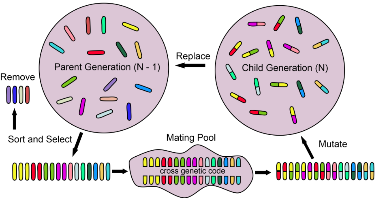
Genetic Algorithms
14
Encoding
Fitness Evaluation
Genetic Operators
p_i =\\ \{x_1, x_2, \dots, x_n\}
f_i =F(p_i)
Improving Chemical Accuracy, for Less
Computational Cost
Accuracy
Machine Learning
16

Regression in Chemistry
17

Replace expensive electronic structure calculation with cheaper, data-driven regression model
\left < \Psi| \hat H | \Psi \right >\rightarrow f(\{Z, R\})

Motivating Remarks
18
1. Searching Chemical Space
2. Improving Chemical Accuracy, for Less
EVOLVE: An Evolutionary Toolbox for the Design of Peptides and Proteins
Nicholas J. Browning, Marta A. S. Perez, Elizabeth Brunk, Ursula Roethlisberger, in submission, JCTC, 2019.
- Introduction
- Motivation
- EVOLVE
- GAML
- ML-MTS

Haemoglobin (PDB 1A3N)
- DNA Signalling
- Acid-base catalysis
- atom/group transfer
- Electron transfer
- Redox catalysis
Design of proteins is attractive:
- Tune or change activity
- Improve solvent tolerance
- Increase thermal stability
Proteins fulfill a wide scope of biological functions ranging from regulation to catalytic activity:
Protein Design
Issues:
- Search space is large
- E.g 50-residue protein:
20^{50} \approx 1 \times 10^{65}
possible sequences
20

Short 20-mer polyalanine
Central 8 residues open to mutation (purple spheres)
EVOLVE Algorithm and Prototype


Side chain dihedrals discretised into set of 177 low-energy conformers [1]
1. Proteins, 2000, 40, pp 389-408
21
\vec{\chi} = \{\chi_i\}
f = \Delta E^\text{mutant}_{\text{system}} - \Delta E^{\text{ref}}_\text{system} = E^\text{mutant}_\text{system} - E^\text{ref}_\text{system} + \sum_i^N (E^{\text{ref}}_\text{aa}(i) - E^{\text{mutant}}_\text{aa}(i))
E_\text{system} = E^{FF99SB}_\text{system} + \Delta G^{GB}_{sol}
Amber FF99SB force field
Solvent effects modelled by implicit solvent model
Backbone stability measure
\epsilon = 80
\epsilon = 5
0
\epsilon = 10
Buried Protein Environment
Solvent Exposed
Intermediary
EVOLVE Fitness Function
22

94 Rotamers
177 Rotamers
177 Rotamers
-40.6 kcal/mol
-28.4 kcal/mol
-42.3 kcal/mol
EVOLVE Optimisation Curves
23

Selection probabilities show consistent convergence towards a subset of chemical space
Selection Probabilities
24


Can use this subset to focus GA exploration on more interesting regions
55 Rotamer subset of residues: TRP, GLU, ASP, HIP, ARG
New fitness: -42.4 kcal/mol
Subspace Search
25
Outlook


J. Am. Chem. Soc., 2018, 140, 13, pp 4517–4521
Mutant protein solvent and pH tolerant
Thermostability greatly increased compared to wild-type
B1 Domain Protein G
26
1. Searching Chemical Space
2. Improving Chemical Accuracy, for Less
Genetic Optimisation of Training Sets for Improved Machine Learning Models of Molecular Properties
Nicholas J. Browning, Raghu Ramakrishnan, O. Anatole von Lilienfeld, Ursula Roethlisberger, JPCL, 2017
- Introduction
- Motivation
- EVOLVE
- GAML
- ML-MTS
-
Can the error be improved by intelligent sampling - is less more?
-
Are there systematic trends in “optimal” training sets?
Chemical Interpolation
29
Chemical Database
8 heavy-atom subset of the QM-9 database [2]
10 thermochemical and electronic properties computed with DFT/B3LYP
2. Sci. Data, 2014, 1.

Out-of-sample test error used as fitness metric
Complex optimisation problem:
Database QM-8
Kernel Ridge Regression
\approx 10^{1449}
C(10900, 1000)
30


Significant reduction in out-of-sample errors
Fewer training molecules required to reach given accuracy
random sampling
GA optimised
Learning Curves - Enthalpy of Atomisation
31
Direct Learning
Delta Learning
Systematic Trends - Moments of Inertia
32

Certain molecules are more representative
Systematic shifts in distance, property, and shape distributions


Systematic Trends - Property Distributions
33
Certain molecules are more representative
Systematic shifts in distance, property, and shape distributions
Motivating Remarks
1. Searching Chemical Space
2. Improving Chemical Accuracy, for Less
34
Machine Learning Enhanced Multiple Time Step Ab Initio Molecular Dynamics
Nicholas J. Browning, Pablo Baudin, Elisa Liberatore, Ursula Roethlisberger, In Submission, 2019
- Introduction
- Motivation
- EVOLVE
- GAML
- ML-MTS
Molecular Dynamics
Provides a 'window' into the microscopic motion of atoms in a system
F_A = -\nabla_A E_0(\{R, r\})
Forces acting on (classical) nuclei calculated from a potential energy surface
36
Key Issues
- Accuracy of the potential energy surface : ML
- Timestep used to integrate atomic forces : MTS
F_A = M_A a(t)
r_A(\Delta t), v_A(\Delta t)
Multiple Time Step Integrators
Address the time step issue by observing that the forces acting on a system have different timescales
Separate "fast" and "slow" components of the total force, which can be integrated using smaller and larger timesteps
37
F_A
F_A^\text{slow}
F_A^\text{fast}
Fast forces: cheap to compute
Slow forces: expensive to compute
MTS Algorithm
\gamma = (r_1, r_2, \dots, r_N, p_1, p_2, \dots, p_N)
iL = iL_\text{fast} + iL_\text{slow}
a(\gamma_t) = e^{iLt}a(\gamma_0)
e^{iL\Delta t} \approx e^{iL_{slow} \frac{\Delta t}{2}} \times e^{iL_\text{fast}\Delta t} (\Delta t) \times e^{iL_{slow} \frac{\Delta t}{2}}
e^{iL\Delta t} \approx e^{iL^\text{slow} (\Delta t/2)} \Big[ e^{iL^\text{fast} (\Delta t/n)} \Big]^n e^{iL^\text{slow} (\Delta t/2)}
Propagatation of phase space vector
Separate slow and fast components
phase space vector
Discrete time propagator obtained from Trotter factorisation
# initialise r, p
dt = 0.36
Dt = dt*n
Fslow = compute_slow_forces(r)
Ffast = compute_fast_forces(r)

for t in range(0, total_time, Dt):
  p = p + 0.5*Dt*Fslow # Integrate slow components

  for i in range(1, n):  # Integrate fast components
    p = p + 0.5*dt*Ffast
    r = r + dt * p/m
    Ffast = compute_fast_forces(r)
    p = p + 0.5*dt*Ffast

  Fslow = compute_slow_forces(q)
  p = p + 0.5*Dt*Fslow # Integrate slow components
38
\delta t
Ab Initio MTS

39
Computational Cost
Accuracy
LDA
PBE0
fast
slow
Machine Learning Potentials
Replace expensive electronic structure method with data-driven kernel model
Delta-learning model naturally results in an MTS scheme
F^\text{fast} = F^\text{low}
F^\text{slow} = \Delta F^\text{ML}
F^\text{fast} = F^\text{low} + \Delta F^\text{ML}
F^\text{slow} = F^\text{high} - F^\text{fast}
Scheme I ML-MTS
Scheme II ML-MTS
\Delta F^\text{ML} = F^\text{high} - F^\text{low}
Exact slow forces
Cost of high level, evaluated infrequently
Approximate slow forces
Cost of low level
40
\Delta E^\text{ML}(M_i) = E^\text{high}(M_i) - E^\text{low}(M_i) = \sum_{I\in i}\sum_{J} k(M_I, M_J) \alpha_J
\Delta F_L^\text{ML}(M_i) = -\frac{\partial \Delta E^\text{ML}}{\partial R_L}(M_i) = -\sum_{I\in i}\sum_J \frac{\partial k(M_I, M_J)}{\partial M_I} \frac{\partial M_I}{\partial R_L} \alpha_J
Use a computationally efficient kernel method [3]:
- Generalisable
- No 2nd derivatives required, only kernel and descriptor gradients
Representation:
-
Atomic environments: Atomic Spectrum of London-Axilrod-Teller-Muto representation (aSLATM) [4]
MPI-ML code implemented into CPMD
Machine Learning Potentials
3. Chem. Phys., 2019, 150, 064105
4. ArXiv, 2017, https://arxiv.org/abs/1707.04146
41
Training Data
Trajectories of small isolated N-water molecule clusters
Fast components = LDA
Slow components = PBE0 - LDA
Predictions made on liquid water


42
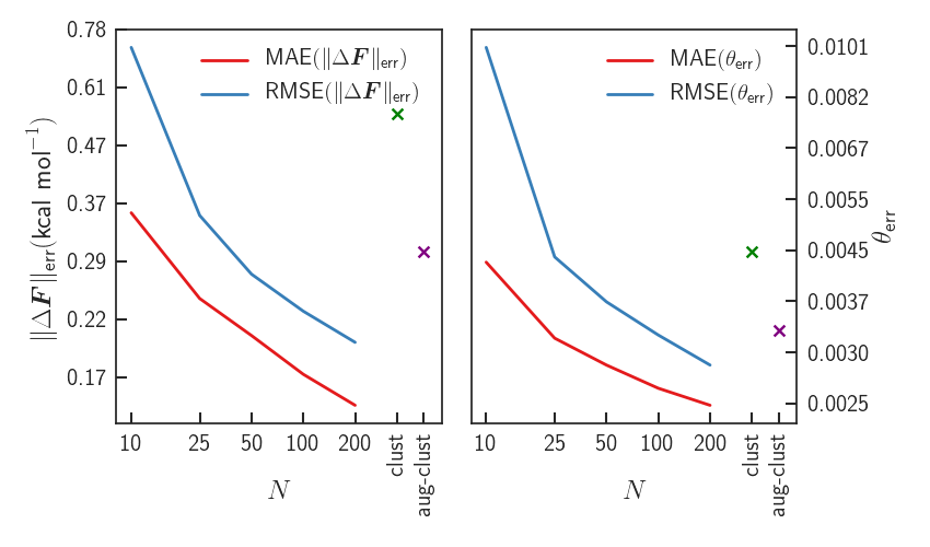
Results - Errors
43

Significant improvement upon LDA - forces almost identical to PBE0

Results - Time Step and Speedup
Significant increase in outer timestep wrt. standard MTS
Resonance effects limit maximum outer timestep
Encouraging increase in overall speedup
Speedup dictated by number of SCF cycles to converge wfn
\epsilon = \frac{1}{N}\sum_i \frac{E_i - \bar{E}}{\bar E}
44
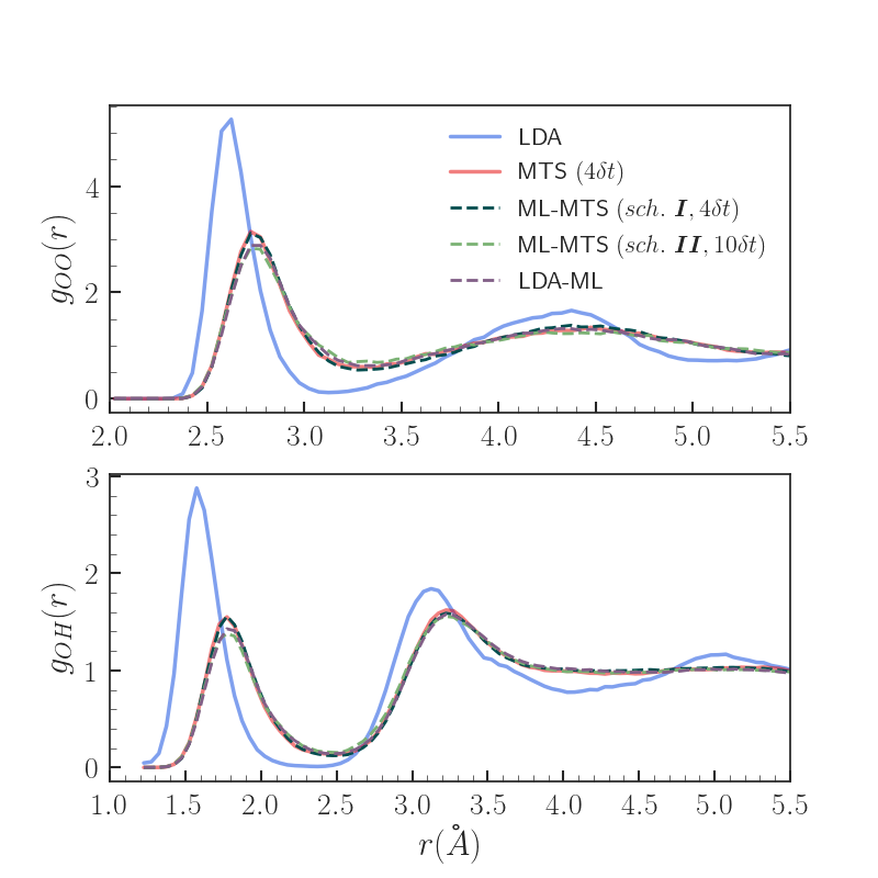
Results - Properties
MTS (n=4dt) identified as yielding properties with excellent agreement wrt. VV-PBE0 in previous work [5]
Both scheme I and II ML-MTS result in significantly improved radial distributions
5. J. Chem. Theory Comput., 2018, 14, 6, pp 2834–2842
45
1. Searching Chemical Space
Conclusions
- EVOLVE is capable of searching through inordinately large chemical spaces
- Meaningful chemical space insights can be gained from the EVOLVE procedure
- Potential for experimental reach
46
2. Improving Chemical Accuracy, for Less
-
Within a specified chemical space, the accuracy of ML models can be significantly improved with intelligent sampling
-
kernel methods can provide a significant increase in timestep used in MTS integrators
- Maintain good accuracy
- Significantly reduce computational cost
Acknowledgements and Thanks


Dr. Raghu Ramakrishnan
Dr. Esra Bozkurt
Dr. Marta A. S. Perez
Dr. Pablo Baudin
Dr. Elisa Liberatore
Prof. Ursula Roethlisberger


Prof. O. Anatole von Lilienfeld
Prof. Clemence Corminboeuf
Dr. Albert Bartók-Pártay
Dr. Ruud Hovius
Acknowledgements and Thanks

Karin Pasche
Family


Family


Family


Family


Diana


LCBC


Cool Dudes and Dudettes


Cheers!
Chemistry
3


Computational Chemistry
42 electrons in 21 orbitals
\hat{H}_e \Psi_e(\vec{r}) = E_e \Psi_e(\vec{r})
- 100 points per orbital
- 8 bytes / point
\rightarrow 800^{21*3} \approx 8\times 10^{182}
bytes
Its terrible...
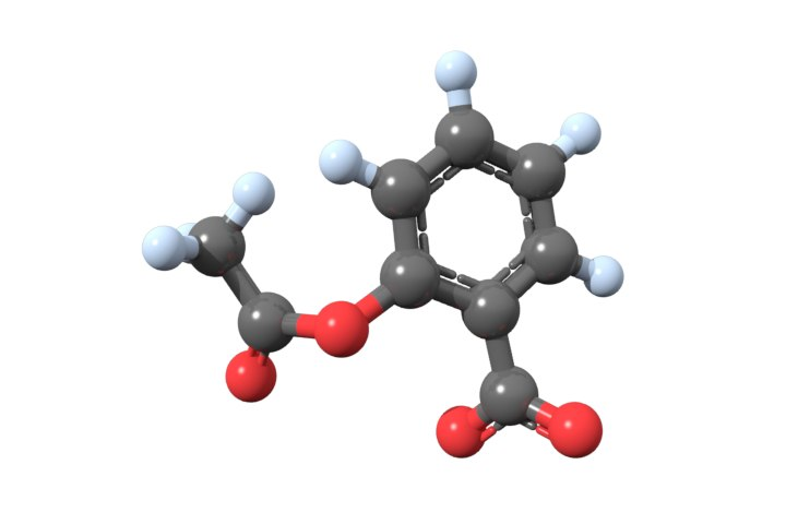
Benzene
\text{C}_6\text{H}_{6}
e
e
e
e
e
e
e
e
e
e
e
e
GA-ML Small Optimal Training Sets
44

GA-ML Distance Distributions
45
\boldsymbol{M}_I^{(2)}(r) = \frac{1}{2} \sum_{J\ne I} Z_IZ_J \frac{1}{\sigma_r \sqrt{2\pi} r^6} e^{-\frac{\left \lVert r - R_{IJ} \right \rVert ^2}{2\sigma_r^2}}
\boldsymbol{M}_I^{(3)}(\theta)= \frac{1}{3}\sum_{I \ne J \ne K} Z_I Z_J Z_K \frac{1}{\sigma_\theta \sqrt{2\pi}} e^{-\frac{\left ( \theta - \theta_{IJK} \right )^2}{2\sigma_\theta^2}} \frac{1 + \cos\theta \cos\theta_{JKI}\cos\theta_{KIJ}}{\left (R_{IJ} R_{IK} R_{KJ}\right)^3}
\boldsymbol{M}_I = \left \{ \boldsymbol{M}^{(1)}_I, \boldsymbol{M}^{(2)}_I, \boldsymbol{M}^{(3)}_I\right \}
SLATM Parameters
46
R_c = 4.8 A
\theta_\text{min} = -0.35 \ \text{rad}
\theta_\text{max} = 3.5 \ \text{rad}
\text{grid resolution}= 0.1A
\text{angular grid resolution}= 0.1
\ \text{rad}
Two-body term:
Three-body term:
\sigma_r = 0.05
\sigma_{\theta} = 0.05
Public: Applications of Artificial Intelligence to Computational Chemistry
By Nick Browning


