training neural networks with orthogonal weights
Pierre Ablin
Apple
Reference:
P. Ablin and G. Peyré. Fast and accurate optimization on the orthogonal manifold without retraction. AISTATS 2022.
P. Ablin, S. Vary, B. Gao and P.-A. Absil. Infeasible Deterministic, Stochastic, and Variance-Reduction Algorithms for Optimization under Orthogonality Constraints. Preprint.
Orthogonal weights in a neural network ?
Orthogonal matrices
A matrix \(W \in\mathbb{R}^{p\times p}\) is orthogonal if and only if (equivalent definitions):
Operator definition:
- $$W^\top W = I_p$$
Norm preservation definition:
- For all \(x\in\mathbb{R}^p\), we have \(\|Wx\| = \|x\|\)
applications in Neural networks
Adversarial robustness: training robust neural networks
Stable training: avoid gradient explosion / vanishing
Generative modelling: a building block for normalizing flows
Robust neural networks
Trained without care, a neural network \(\phi_{\theta}\) is not robust: it is susceptible to adversarial attacks

Goodfellow, Ian J., Jonathon Shlens, and Christian Szegedy. "Explaining and harnessing adversarial examples."
Robust neural networks
Trained without care, a neural network \(\phi_{\theta}\) is not robust: it is susceptible to adversarial attacks
For an input \(x\) we can find a small perturbation \(\delta\) such that
$$\|\phi_{\theta}(x+\delta) - \phi_{\theta}(x)\| \gg \|\delta\|$$
One remedy: certified robustness
Idea: if we can ensure that a neural network is Lipschitz, then it is robust.
For instance
$$\sup_{x, \delta} \frac{\|\phi_{\theta}(x + \delta) - \phi_\theta(x)\|}{\|\delta\|} \leq 1$$
Critical remark: the composition of 1-Lipschitz maps is 1-Lipschitz
To construct a 1-Lipschitz neural network, it suffices to stack 1-Lipschitz layers !
1-Lipschitz
1-Lipschitz
1-Lipschitz
1-Lipschitz
Cisse, et al. "Parseval networks: Improving robustness to adversarial examples.", 2017
Li et al. "Preventing gradient attenuation in Lipschitz constrained convolutional networks.", 2019
Lipschitz layers with orthogonal matrices
Consider the transform
$$x\mapsto Wx$$with \(W\in\mathbb{R}^{p\times p}\) is such that \(W^\top W =I_p\)
This is a norm preserving layer, hence 1-Lipschitz: can be used as a building block for certified robustness networks.
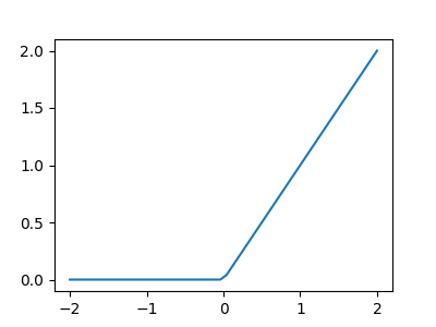
We can then stack this transform with other 1-Lipschitz layers, such as
\(x\mapsto \mathrm{ReLU}(x)\)
Gradient explosion
Consider a sequence of transforms
$$x_{n+1} = \sigma(W_nx_n + b_n), $$
with \(W_n\) some matrices, for \(L\) layers.
By the chain rule:
$$\frac{\partial x_L}{\partial x_n} =\prod_{k=n}^{L-1}D_k W_k^\top,\enspace\text{with } D_k = \mathrm{diag}(\sigma'(W_kx_k +b_k))$$
Bounding this:
$$\|\frac{\partial x_L}{\partial x_n} \|_2\leq \prod_{k=n}^{L-1}\|D_k\|_2\|W_k\|_2$$
If the weights are orthogonal and \(\sigma\) is a ReLU:
$$\|\frac{\partial x_L}{\partial x_n} \|_2\leq 1$$
Avoids gradient explosion !

Generative modelling
Generative modelling:
Samples \(x_1, \dots, x_n\sim p\).
Goal: get new samples from distribution \(p\)
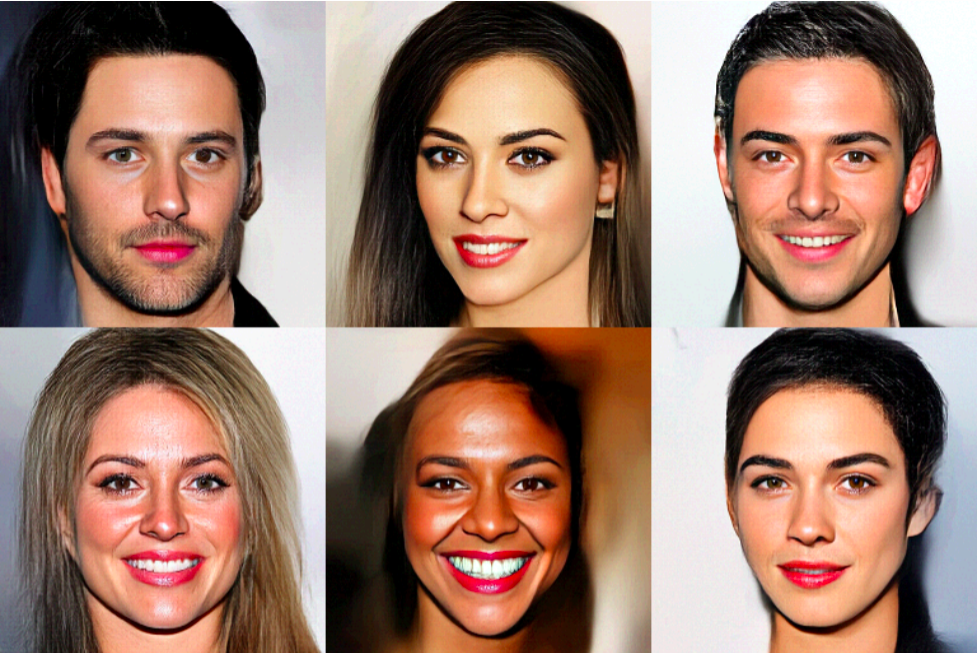
Example on faces data
Normalizing flows
Idea: use a probabilistic model
$$x = g_{\theta}(z), \enspace \text{with }z\sim \mathcal{N}(0, I_p)$$
where the function \(g_{\theta}\) is invertible
Find parameters by maximum likelihood: Letting \(f_\theta = g_{\theta}^{-1}\),
$$\log(p(x)) = \log|\frac{\partial f_{\theta}(x)}{\partial x}| + \log(p(z))$$
Gaussian so simple


$$g_{\theta}$$
$$f_{\theta}$$
$$z$$
$$x$$
Invertible neural networks
$$x = g_{\theta}(z), \enspace \text{with }z\sim \mathcal{N}(0, I_p)$$
where the function \(g_{\theta}\) is invertible
How to build invertible neural networks ?
- Orthogonal matrices are easily inverted, with stable inversion
$$\text{For } W\text{ orthogonal, }y =Wx \Leftrightarrow x = W^{\top}y$$
- We can stack orthogonal layers and simple activation functions
Training neural networks with orthogonal weights
Training problem
Neural network \(\phi_{\theta}: x\mapsto y\) with parameters \(\theta\). Some parameters are orthogonal matrices.
Dataset \(x_1, \dots, x_n\).
Find parameters by empirical risk minimization:
$$\min_{\theta}f(\theta) = \frac1n\sum_{i=1}^n\ell_i(\phi_{\theta}(x_i))$$
\(\ell_i\) individual loss function (e.g. log-likelihood, cross-entropy with targets, ...)
How to do this with orthogonal weights?
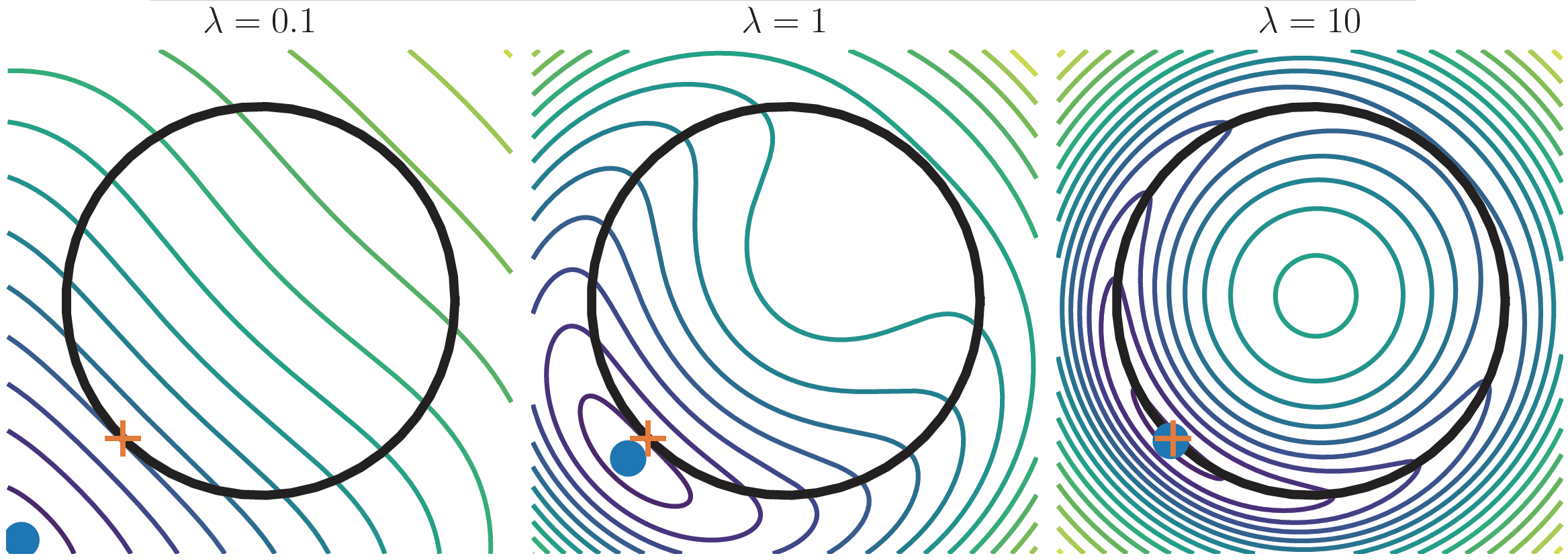
penalty method?
Simple method to get approximal orthogonality:
$$\min f(M) + \lambda \|M^{\top}M-I_p\|^2$$
- Simple
- Can use Adam on top
- Not perfect orthogonality
- To get close to orthogonality, need high \(\lambda\), which gives bad conditioning
Orthogonal manifold
\( \mathcal{O}_p = \{W\in\mathbb{R}^{p\times p}|\enspace W^\top W =I_p\}\) is a Riemannian manifold:
Around each point, it looks like a linear vector space.
Problem:
$$\min_{W\in\mathcal{O}_p}f(W)$$
Two main approaches:
\mathcal{O}_p
Classical
Extend Euclidean algorithms to the Riemannian setting (gradient descent, stochastic gradient descent,...)
Trivializations
Transform the manifold into a linear space \(E\) and then optimize on this space
E
Optimization on the orthogonal manifold 101
\mathcal{O}_p
Euclidean Gradient descent:
$$W' = W- \eta \nabla f(W)$$
Not tangent
Goes out of \(\mathcal{O}_p\)
W
-\nabla f(W)
Absil, P-A., Robert Mahony, and Rodolphe Sepulchre. Optimization algorithms on matrix manifolds.
Tangent space
\mathcal{O}_p
W
-\nabla f(W)
\(T_W\) : tangent space at \(W\).
Set of all tangent vectors at \(W\).
T_W
For \(\mathcal{O}_p\), global equation:
$$WW^\top = I_p$$
By differentiation:
$$\dot W W^\top + W{\dot W}^\top = 0$$
Tangent space:
$$T_W = \{Z\in\mathbb{R}^{p\times p}|\enspace ZW^\top + WZ^\top = 0\}$$
$$T_W = \mathrm{Skew}_p W$$
Set of skew-symmetric matrices
Riemannian gradient
\mathcal{O}_p
W
-\nabla f(W)
T_W
Tangent space:
$$T_W = \{Z\in\mathbb{R}^{p\times p}|\enspace ZW^\top + WZ^\top = 0\}$$
$$T_W = \mathrm{Skew}_p W$$
Riemannian gradient:
$$\mathrm{grad}f(W) = \mathrm{proj}_{T_W}(\nabla f(W)) \in T_W$$
-\mathrm{grad} f(W)
On \(\mathcal{O}_p\):
$$\mathrm{grad}f(W) = \mathrm{Skew}(\nabla f(W)W^\top) W$$
Projection on the skew-symmetric matrices: \(\mathrm{skew}(M) = \frac12(M - M^\top)\)
Knowing \(\nabla f(W)\), need 2 matrix-matrix multiplications to compute it
Riemannian gradient flow
\mathcal{O}_p
W
-\nabla f(W)
T_W
Riemannian gradient:
$$\mathrm{grad}f(W) = \mathrm{proj}_{T_W}(\nabla f(W))$$
-\mathrm{grad} f(W)
Allows to define the Riemannian gradient flow
$$\dot W(t) = -\mathrm{grad}f(W(t)),\enspace W(0)\in\mathcal{O}_p$$
Easy to show \(W(t)\in\mathcal{O}_p\) for all \(t\):
- Flow stays on the manifold
Convergence to critical points of \(f\)
DiscrEtization
\mathcal{O}_p
W
-\nabla f(W)
T_W
-\mathrm{grad} f(W)
Riemannian gradient flow
$$\dot W(t) = -\mathrm{grad}f(W(t)),\enspace W(0)\in\mathcal{O}_p$$
Euler discretization
$$W^{t+1} = W^t - \eta \mathrm{grad}f(W^t)$$
Goes out of \(\mathcal{O}_p\) :(
Retractions: moving on the manifold
\mathcal{O}_p
W
T_W
Z
Retraction:
$$\mathcal{R}(W, Z) = W'$$
where:
- \(W\in\mathcal{O}_p\)
- \(Z\in T_W\)
- \(W'\in\mathcal{O}_p\)
and:
$$\mathcal{R}(W, Z) = W+Z + o(\|Z\|)$$
Allows to move on the manifold
\mathcal{R}(W, Z)
Retractions: examples
On \(\mathcal{O}_p\), \(T_W = \mathrm{Skew}_pW\), hence for \(Z\in T_W\) we can write
$$Z = AW,\enspace A^\top = -A$$
Classical retractions :
- Exponential: \(\mathcal{R}(W, AW) =\exp(A)W\)
- Cayley: \(\mathcal{R}(W, AW) =(I -\frac A2)^{-1}(I + \frac A2)W\)
- Projection: \(\mathcal{R}(W, AW) = \mathrm{Proj}_{\mathcal{O_p}}(W + AW)\)
\mathcal{O}_p
W
T_W
Z
\mathcal{R}(W, Z)
Riemannian gradient descent
\mathcal{O}_p
W^0
-\mathrm{grad} f(W^0)
- Start from \(W_0\in\mathcal{O}_p\)
- Iterate \(W^{t+1} = \mathcal{R}(W^t, -\eta\mathrm{grad} f(W^t))\)
W^1
-\mathrm{grad} f(W^1)
-\mathrm{grad} f(W^2)
W^2
W^3
Extensions
Riemannian gradient descent:
- Start from \(W_0\in\mathcal{O}_p\)
- Iterate \(W^{t+1} = \mathcal{R}(W^t, -\eta\mathrm{grad} f(W^t))\)
Riemannian stochastic gradient descent:
- Start from \(W_0\in\mathcal{O}_p\)
- Iterate \(W^{t+1} = \mathcal{R}(W^t, -\eta\mathrm{grad} f_i(W^t))\) with \(i\sim \{1, n\}\)
Empirical risk minimization:
$$f(W) = \frac1n\sum_{i=1}^nf_i(W)$$
Possible to develop accelerated variants (like momentum) but not trivial
Trivializations
Idea: find a surjective map \(\phi: E \to \mathcal{O}_p\) where \(E\) is a vector space
$$\min_{W\in\mathcal{O}_p} f(W)$$
$$\min_{M\in E} f(\phi(M))$$
\mathcal{O}_p
E
\phi
We can then use any classical optimization algorithm to minimize \(f\circ \phi\) !
Practical for deep learning where we want to use ADAM, RMSProp...
For instance \(E = \mathrm{Skew}_p\) and \(\phi(M) =\exp(M)\)
| Lezcano Casado, Mario. "Trivializations for gradient-based optimization on manifolds." NeurIPS 19. |
Today's problem: these methods are often very costly for deep learning
COmputational cost 1
Riemannian gradient descent in a neural network:
- Compute \(\nabla f(W)\) using backprop
- Compute the Riemannian gradient \(\mathrm{grad}f(W) = \mathrm{Skew}(\nabla f(W)W^\top)W\)
- Move using a retraction \(W\leftarrow \mathcal{R}(W, -\eta \mathrm{grad} f(W))\)
Classical retractions :
- Exponential: \(\mathcal{R}(W, AW) =\exp(A)W\)
- Cayley: \(\mathcal{R}(W, AW) =(I -\frac A2)^{-1}(I + \frac A2)W\)
- Projection: \(\mathcal{R}(W, AW) = \mathrm{Proj}_{\mathcal{O_p}}(W + AW)\)
These are:
- costly linear algebra operations
- not suited for GPU (hard to parallelize)
- can be the most expensive step
COmputational cost 2
Trivializations in a neural network:
- Compute \(\nabla\left( f(\phi(M))\right)\) using backprop
- Do a gradient descent step on this function
Problem:
$$\nabla\left( f(\phi(M)) \right) = \left(\frac{\partial \phi}{\partial M}\right)^{\top}\nabla f(\phi(M))$$
Very costly vector-Jacobian product!
If \(\phi = \exp\), need to compute the \(\exp\) of a \(2p\times 2p\) matrix...
Rest of the talk: find a cheaper alternative
Main idea
In a deep learning setting, moving on the manifold is too costly !
Can we have a method that is free to move outside the manifold that
- Still converges to the solutions of \(\min_{W\in\mathcal{O}_p} f(W)\)
- Has cheap iterations ?
Spoiler: yes !
Projection "paradox''
\mathcal{O}_p
Take a matrix \(M\in\mathbb{R}^{p\times p}\)
It is cheap and easy to check if \(M\in\mathcal{O}_p\).
M
Just compute \(\|MM^\top - I_p\|\) and check if it is close to 0.
But projecting \(M\) on \(\mathcal{O}_p\) is expensive:
$$\mathcal{Proj}_{\mathcal{O}_p}(M) = (MM^\top)^{-\frac12}M$$
\mathcal{Proj}_{\mathcal{O}_p}(M)
Projection "paradox''
\mathcal{O}_p
Take a matrix \(M\in\mathbb{R}^{p\times p}\)
It is cheap and easy to check if \(M\in\mathcal{O}_p\).
M
Just compute \(\|MM^\top - I_p\|\) and check if it is close to 0.
Idea: follow the gradient of $$\mathcal{N}(M) = \frac14\|MM^\top - I_p\|^2$$
\mathcal{Proj}_{\mathcal{O}_p}(M)
$$\nabla \mathcal{N}(M) = (MM^\top - I_p)M$$
The iterations \(M^{t+1} = M^t - \eta\nabla \mathcal{N}(M^t)\) converge to the projection
Special structure : symmetric matrix times M...
-\nabla \mathcal{N}(M)
optimization and projection
Projection
Follow the gradient of $$\mathcal{N}(M) = \frac14\|MM^\top - I_p\|^2$$
$$\nabla \mathcal{N}(M) = (MM^\top - I_p)M$$
Optimization
Riemannian gradient:
$$\mathrm{grad}f(M) = \mathrm{Skew}(\nabla f(M)M^\top) M$$
These two terms are orthogonal !
The landing field
Projection
Follow the gradient of $$\mathcal{N}(M) = \frac14\|MM^\top - I_p\|^2$$
$$\nabla \mathcal{N}(M) = (MM^\top - I_p)M$$
Optimization
Riemannian gradient:
$$\mathrm{grad}f(M) = \mathrm{Skew}(\nabla f(M)M^\top) M$$
$$\Lambda(M) = \mathrm{grad}f(M) + \lambda \nabla \mathcal{N}(M)$$
\mathcal{O}_p
M
-\nabla \mathcal{N}(M)
-\mathrm{grad}f(M)
\Lambda(M)
The landing field
$$\Lambda(M) = \mathrm{Skew}(\nabla f(M)M^\top) M + \lambda (MM^\top - I_p)M$$
Because of orthogonality of the two terms:
$$\Lambda(M) = 0$$
if and only if
- \(MM^\top - I_p = 0\) so \(M\) is orthogonal
- \(\mathrm{grad}f(M) = 0\) so \(M\) is a critical point of \(f\) on \(\mathcal{O}_p\)
The landing field is cheap to compute
$$\Lambda(M) = \left(\mathrm{Skew}(\nabla f(M)M^\top) + \lambda (MM^\top-I_p)\right)M$$
Only matrix-matrix mutliplications ! No expensive linear algebra + parrallelizable on GPU's
Comparison to retractions:

The Landing algorithm:
$$\Lambda(M) = \left(\mathrm{Skew}(\nabla f(M)M^\top) + \lambda (MM^\top-I_p)\right)M$$
Starting from \(M^0\in\mathcal{O}_p\), iterate
$$M^{t+1} = M^t -\eta \Lambda(M^t)$$
\mathcal{O}_p
M^0
-\mathrm{grad}f(M)
M^1
-\nabla \mathcal{N}(M)
-\mathrm{grad}f(M)
-\mathrm{grad}f(M)
M^2
-\nabla \mathcal{N}(M)
convergence result
$$\Lambda(M) = \left(\mathrm{Skew}(\nabla f(M)M^\top) + \lambda (MM^\top-I_p)\right)M$$
Starting from \(M^0\in\mathcal{O}_p\), iterate
$$M^{t+1} = M^t -\eta \Lambda(M^t)$$
Theorem (informal):
If the step size \(\eta\) is small enough, then we have for all \(T\):
$$\frac1T\sum_{t=1}^T\|\mathrm{grad} f(M^t)\|^2 = O(\frac1T)$$
$$\frac1T\sum_{t=1}^T\mathcal{N}(M^t) = O(\frac1T)$$
Same rate of convergence as classical Riemannian gradient descent
Convergence to \(\mathcal{O}_p\)
Extension to sgd
$$\Lambda_i(M) = \left(\mathrm{Skew}(\nabla f_i(M)M^\top) + \lambda (MM^\top-I_p)\right)M$$
Starting from \(M^0\in\mathcal{O}_p\), iterate
$$M^{t+1} = M^t -\eta \Lambda_i(M^t), \text{ with } i\sim \mathcal{U}[1, n]$$
Empirical risk minimization:
$$f(M) = \frac1n\sum_{i=1}^nf_i(M)$$
We get the same rate as Riemannian SGD
We also develop variance-reduction methods for faster convergence
Experiments
(In each experiment, we take \(\lambda = 1\) )
Procrustes problem
$$f(W) = \|AW - B\|^2,\enspace A, B\in\mathbb{R}^{p\times p}$$
$$p=40$$
Comparison to other Riemannian methods with retractions
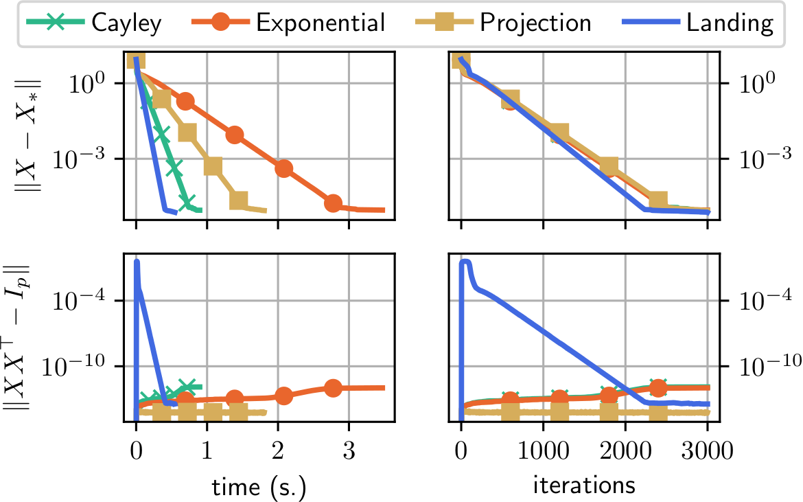
Same convergence curve as classical Riemannian gradient descent
One iteration is cheaper hence faster convergence
Distance to the manifold: increases at first then decreases
Neural networks: distillation
Model: multi-layer perceptron with orthogonal weights
$$x_{n+1} = \sigma(W_nx_n + b_n)$$
Defines a target network \(\phi_{\theta^*}: x_0\to x_L\)
Goal: train a new network from scratch \(\phi_{\theta}\) such that for \(x\) in the training set,
\(\phi_{\theta}(x) \simeq\phi_{\theta^*}(x)\)
$$f(\theta) = \frac1n\sum_{i=1}^n \|\phi_{\theta}(x_i) - \phi_{\theta^*}(x_i)\|^2$$
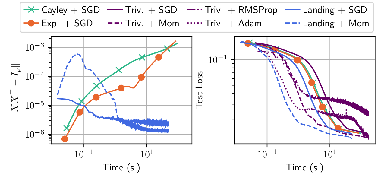
Trivializations are very costly per iterations
Retractions methods drift away from the manifold because of numerical errors accumulations
Neural networks: Training a resnet on cifar
Model: residual network, with convolutions with orthogonal kernels
Trained on CIFAR-10 (dataset of 60K images, 10 classes)
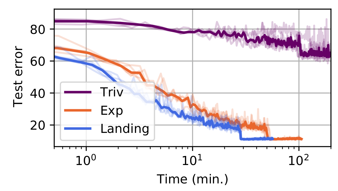
Here trivializations do not work
Conclusion
- Landing method: a cheap, unfeasible method on the orthogonal manifold with strong convergence guarantees
- Useful when retractions are the bottleneck in optimization algorithms
Thanks !
DMA seminar neural nets orthogonal weights
By Pierre Ablin


