Structure of basins of attraction of jammed systems
Praharsh Suryadevara
Mathias Casiulis
Stefano Martiniani


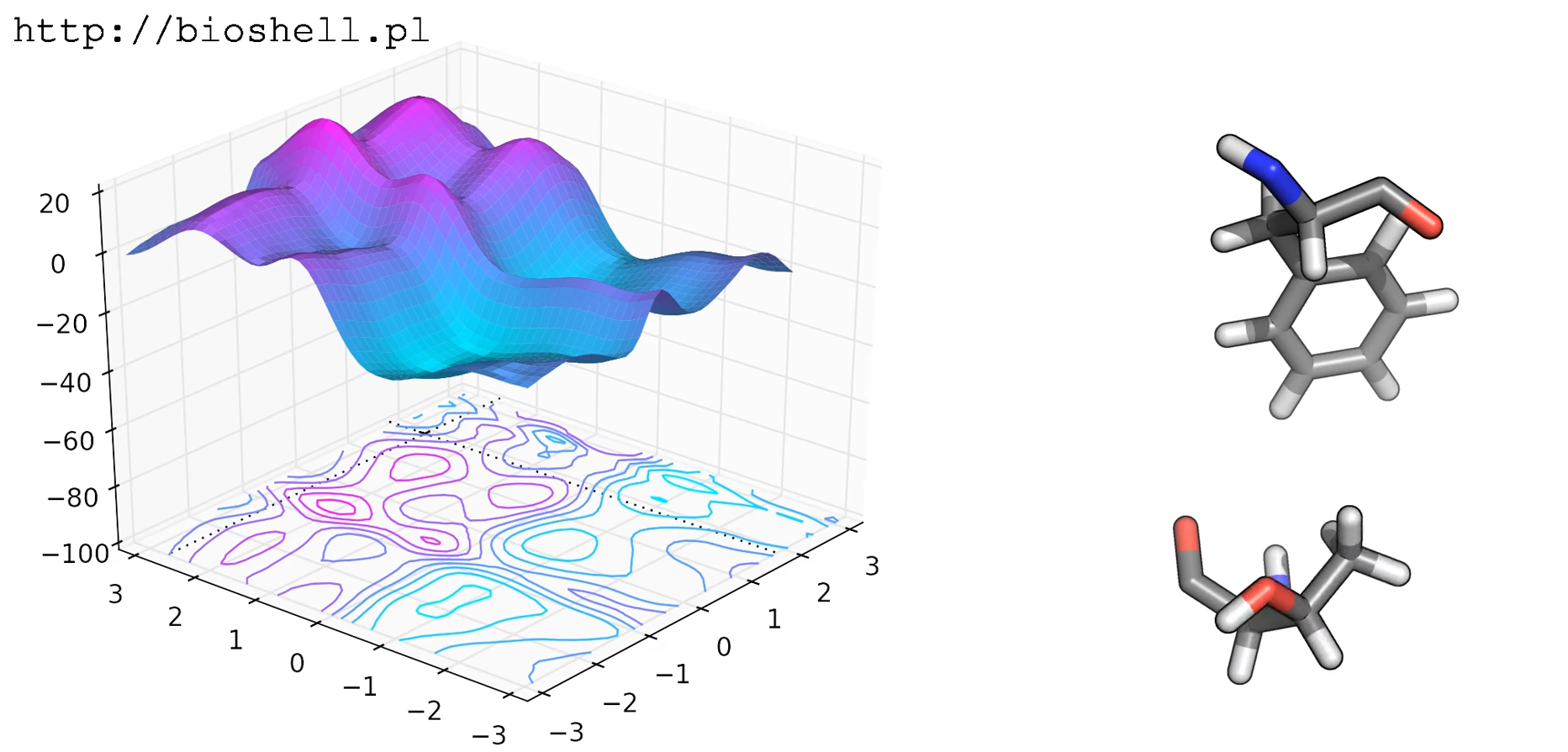
Understanding Energy Landscapes
Energy as a function of conformational angles of a molecule
Energy Landscapes in one dimension

\(V(x)\)
\(x\)
Energy Landscapes in one dimension
\(V(x)\)
\(x\)
\(x_0\)
Energy Landscapes in one dimension
\(V(x)\)
\(x\)
$$ \frac{\text{d} x}{\text{d} t} = - \nabla V(x)$$
Steepest Descent
\(x_0\)
Energy Landscapes in one dimension
\(V(x)\)
\(x\)
$$ \frac{\text{d} x}{\text{d} t} = - \nabla V(x)$$
Steepest Descent
\(x_0\)
Energy Landscapes in one dimension
\(V(x)\)
\(x\)
$$ \frac{\text{d} x}{\text{d} t} = - \nabla V(x)$$
Steepest Descent
\(x_0\)
Energy Landscapes in one dimension
\(V(x)\)
\(x\)
$$ \frac{\text{d} x}{\text{d} t} = - \nabla V(x)$$
Steepest Descent
\(x_0\)
\(x_{min}\)
Energy Landscapes in one dimension
\(V(x)\)
\(x\)
basin 2
Basin tiling (what we're interested in)
basin 1
basin 3
$$ \frac{\text{d} x}{\text{d} t} = - \nabla V(x)$$
Steepest Descent
Basins in high dimensions
Casiulis et al. Papers in Physics 15 (2023): 150001-150001.
Most Volume

Probability of landing inside the basin
Hypercube \(~1000d\)
Basin identification in \((N-1)\times d\) dimensions
$$ \frac{\text{d} x}{\text{d} t} = - \nabla V(x)$$
steepest descent
- Solving steepest descent in \((N-1) \times D\) for interacting potentials is expensive
- Previous work mostly relies on optimization algorithms as proxies for finding basins
Momentum-based optimizers (e.g. FIRE)
Newton/Quasi-Newton methods (e.g. LBFGS)
https://en.wikipedia.org/wiki/Newton%27s_method_in_optimization
Goal of this Talk
I want to show you, with new physics along the way, how to get features of the energy landscape accurately
System
Bidisperse Hertzian soft spheres

$$ V_{ij}(r) =\begin{cases} \frac{\epsilon}{p} \left( 1 - \frac{r}{r_{i} + r_{j}} \right) ^{p} & r < r_{i} + r_{j} \\ 0 & r > r_{i} + r_{j}\end{cases}$$ with \(p\) = 2.5 and packing fraction \(\phi=0.9\) unless otherwise specified

landscape dimension \(d_l \sim (N-1)\times d\)
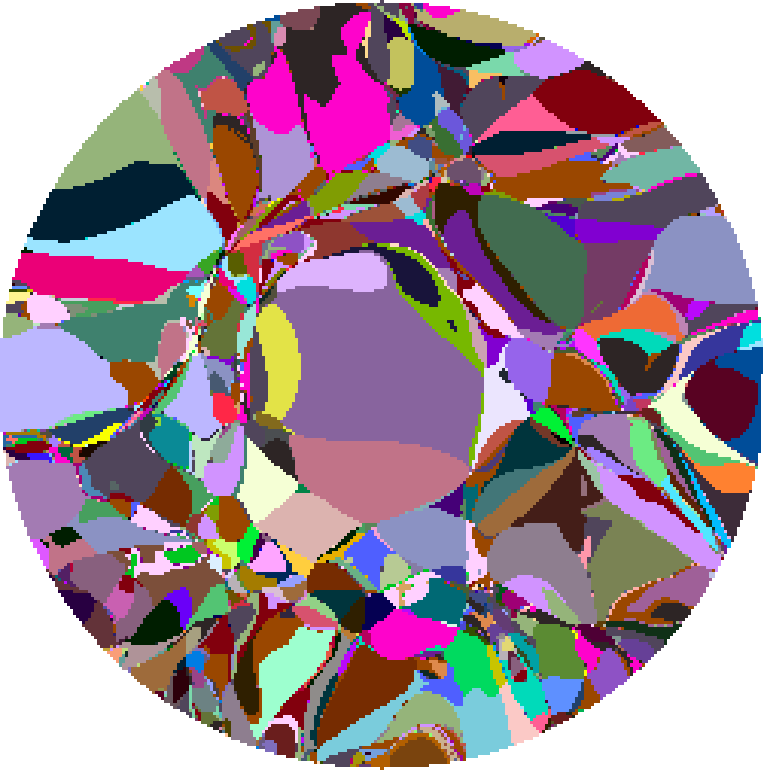
Slicing the energy landscape
Each color is a basin
Imagine cubic basins in a regular grid
Slicing the energy landscape
Each color is a basin
Imagine cubic basins in a regular grid
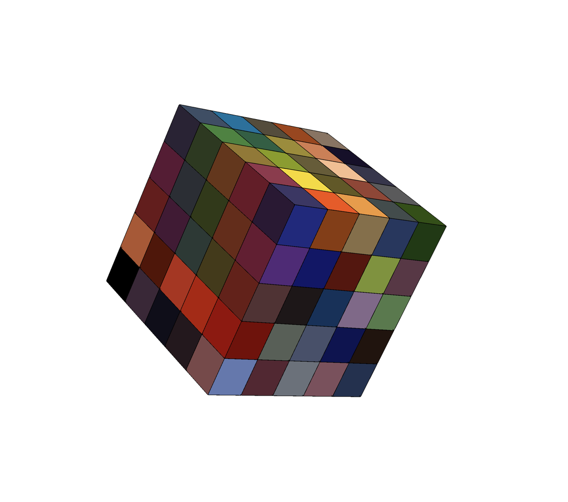
16 particle basin slice with FIRE
16 particle basin slice with FIRE
\(d_l \sim 30\)
\(d_l \sim 30\)
ODE Solver Comparison (1024 particles)
Local error
Time (s)

CVODE (Best)
QNDF
Adaptive Implicit Runge Kutta
Adaptive Implicit Euler
\(\times 10^3\)
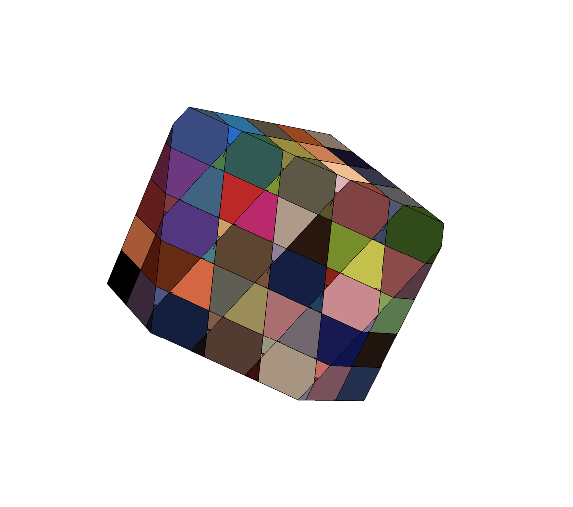
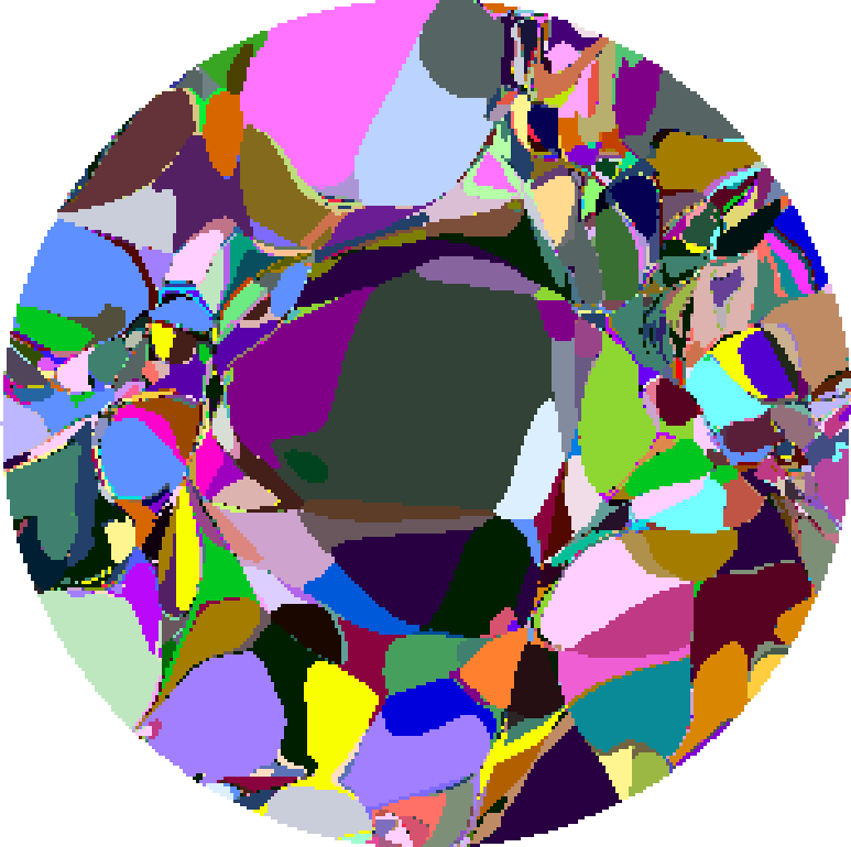
16 particle basin slice with CVODE
16 particle basin slice with CVODE
\(d_l \sim 30\)
\(d_l \sim 30\)
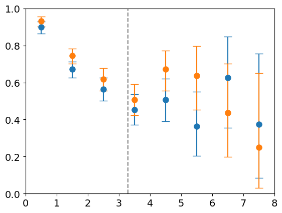
Exact Basins: 8 particles
Accuracy
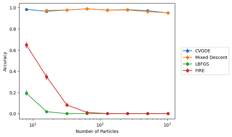
FIRE
LBFGS


FIRE
CVODE
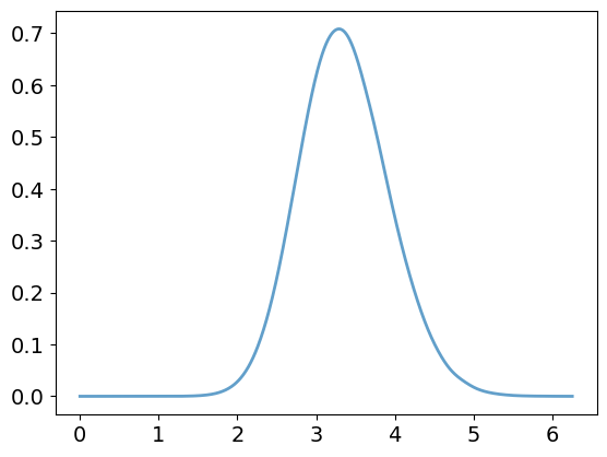
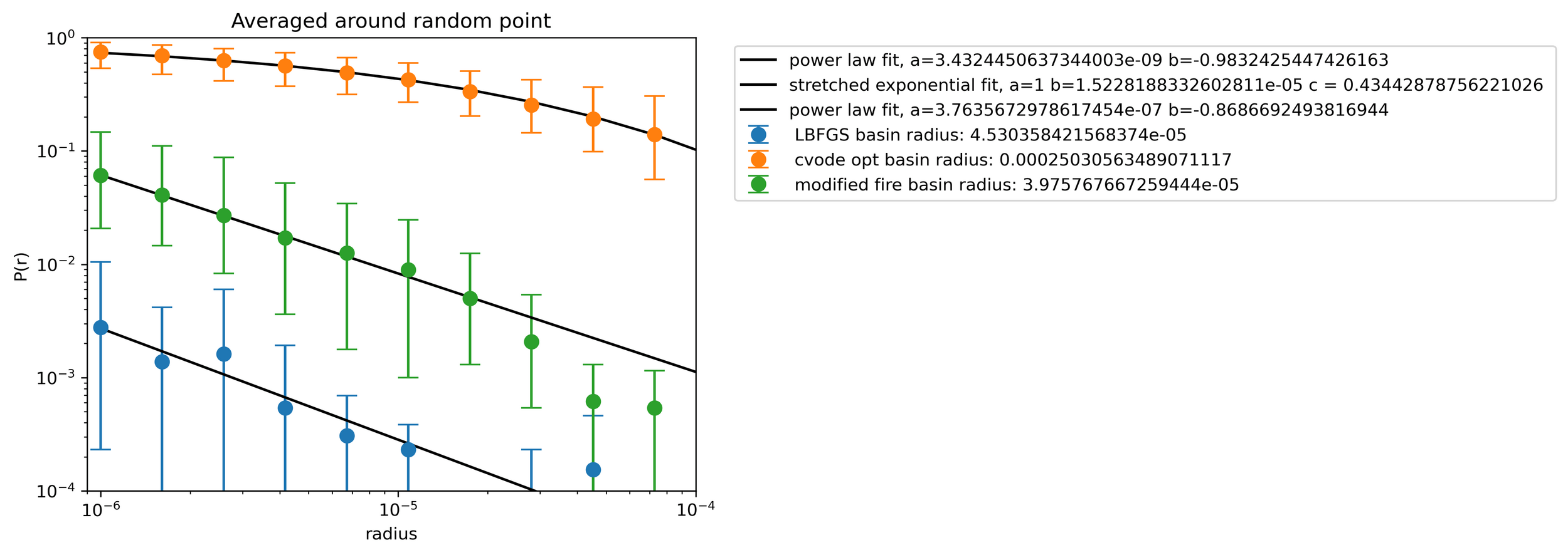
Survival probability in a tentacle
Distance from point
CVODE
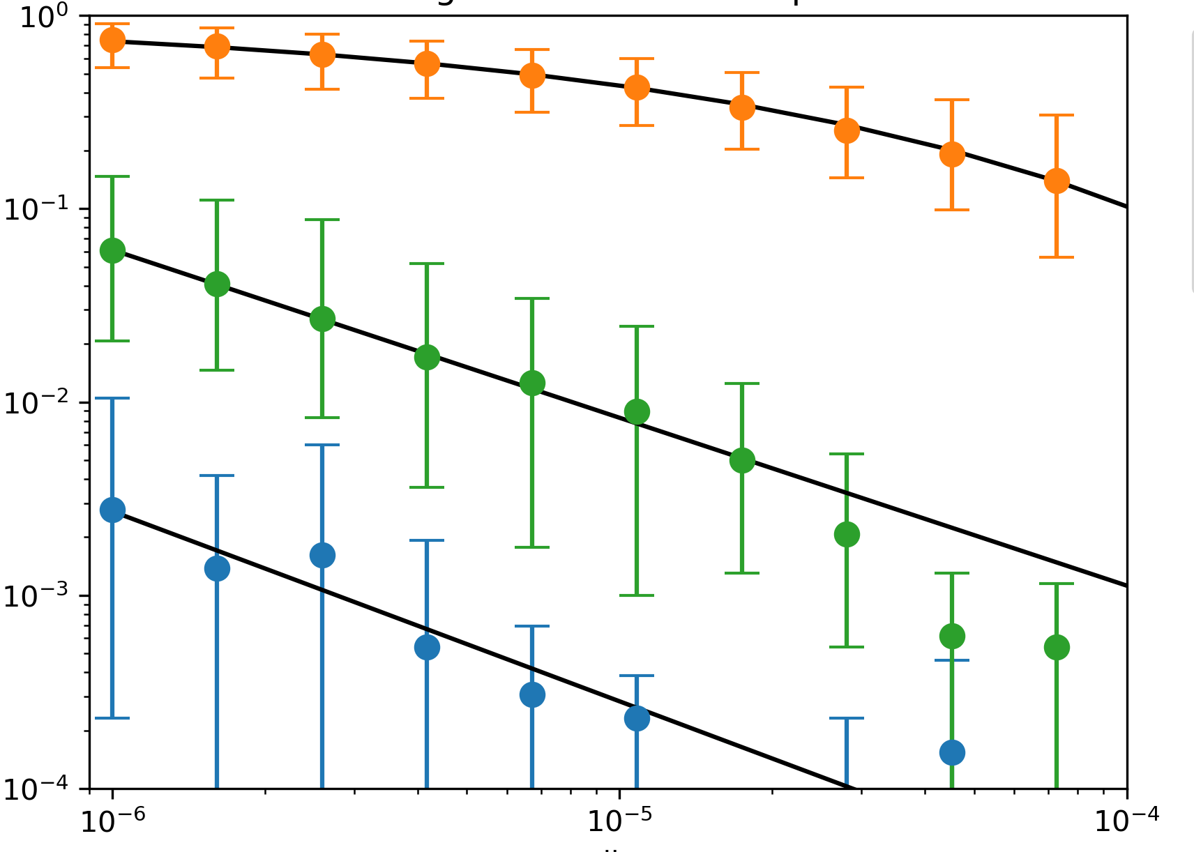
FIRE
LBFGS
\(P(r) = a x^b \)
Survival
Probability
CVODE
\(d_l = 2046 \)
\(P(r)=e^{-(r/r_0)^b}\)
\(1024\) particles
\(P(r) = a x^b \)
CVODE
Accuracy within a single basin
\(8\) particles
\(d_l = 14 \)
LBFGS
FIRE
Distance from minimum
Accuracy
Most basin volume
Distance from minimum
Radial Density of Basin
Optimizer accuracy
Density
Acknowledgments
Martiniani Lab

Stefano Martiniani
Mathias Casiulis
Backup
Calculating volumes in high dimensions
Casiulis et al. Papers in Physics 15 (2023): 150001-150001.


Calculating volumes in high dimensions
Casiulis et al. Papers in Physics 15 (2023): 150001-150001.
$$Z(k) = \int_{\mathbb{R}^N}^{} \mathcal{O}(x) e^{- \frac{1}{2} k \left|x-x_{0}\right|^{2}} dx$$
Partition function
Oracle (1 if inside basin. 0 if outside)
Spring (to control exploration)
$$ F(k) = - log(Z_{k}) $$
Free energy
$$ F(0) - F(k_{\infty}) = \int_{0}^{k_{\infty}} \frac{\partial F}{\partial k} dk = \int_{k_{\infty}}^{0} \langle \left| x-x_{0}\right|^{2} \rangle_{k} dk$$
Log volume (unknown)
Spring free energy
Fit data
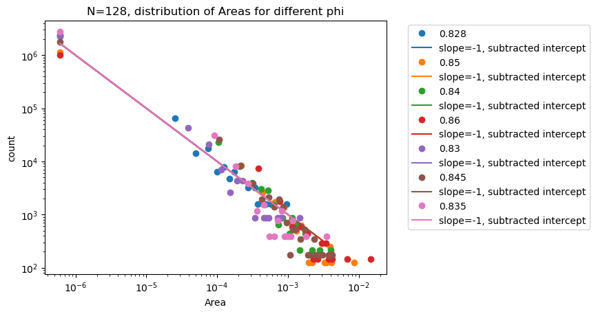
Areas

\(N=128\) \(d_l = 254\)
Polydisperse spheres

\(d_l = 32\)
Hypercubic tiling
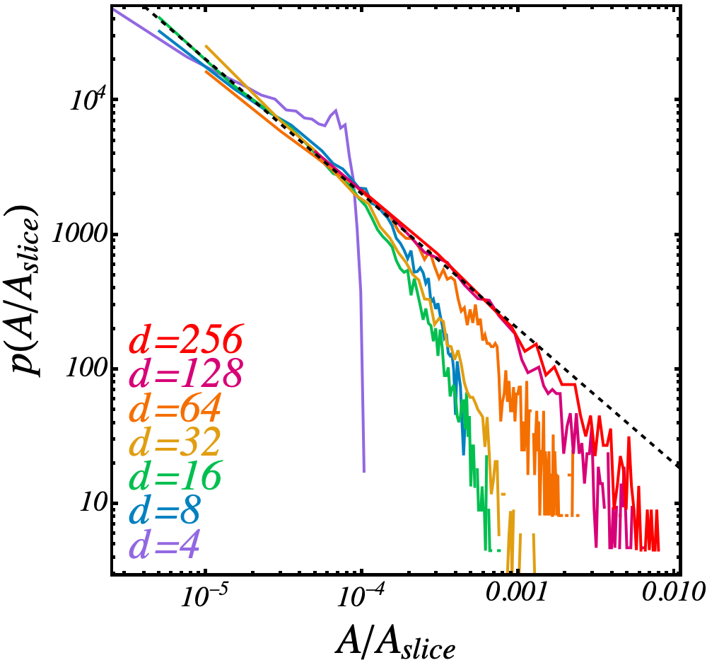
Cubes in high dimensions
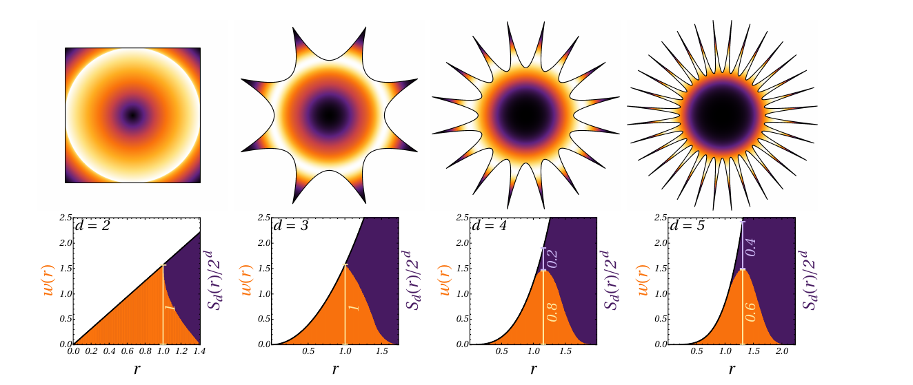
Casiulis et al. Papers in Physics 15 (2023): 150001-150001.
Most volume
Text
Energy Landscapes in one dimension
\(V(x)\)
\(x\)
$$ \frac{\text{d} x}{\text{d} t} = - \nabla V(x)$$
steepest descent
basin 2
Basin Tiling (What we're interested in)
basin 1
basin 3
Can we do better?: Mixed Descent
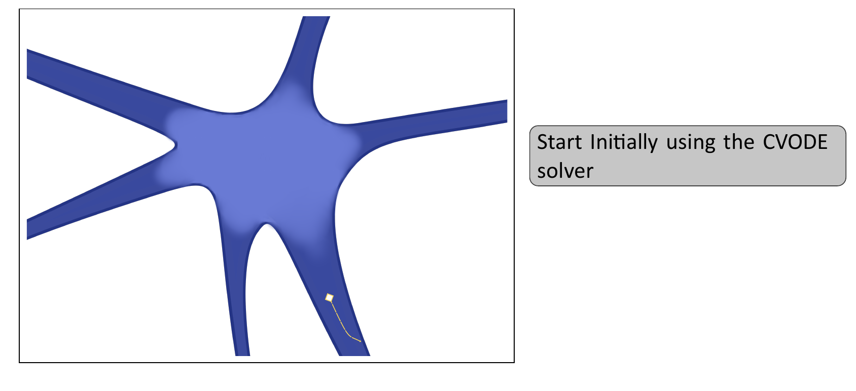
- Start with the CVODE solver
Basin identification
$$ \frac{\text{d} x}{\text{d} t} = - \nabla V(x)$$
steepest descent
- Solving steepest descent in \(nD\) for interacting potentials is hard.
- a large volume of previous work mostly relies on optimization algorithms as proxies for finding basins
Method
- Use CVODE to solve the steepest descent equations
- CVODE is much faster than Gradient descent
- CVODE is much faster than scipy implemented stiff ODE methods
- Identify minima/optimize with pele (https://github.com/martiniani-lab/pele). Hard fork of Wales group code with additional functionality implemented
- Code implemented in basinerror (https://github.com/martiniani-lab/basinerror)
Goals for the talk
- I want to show you how to get basins of attraction in high dimensions accurately
- I want to show you how you can get them fast
Accuracy curves: Harmonic potential (2d)

CVODE: Results
How to get Global Accuracy
- Generate \(N\) steepest descent trajectories to the minima at very low \(rtol\) from random initial conditions
- verify that the minima don't change when you increase \(rtol\) $$\frac{N_\text{incorrect}}{N} < 0.01 $$
\(N\)
\(rtol\)
95 percent accuracy
Accuracy curves: Harmonic potential (2d)
Random cut around the "global maximum"
\( 8 \times \)equilibrum pairwise distance

Random cut around a local minimum
Random cut around a local minimum LJ 13
\( 8 \times \)equilibrum pairwise distance
\( 8 \times \)equilibrum pairwise distance
Colors not matched!!
A fast and accurate algorithm
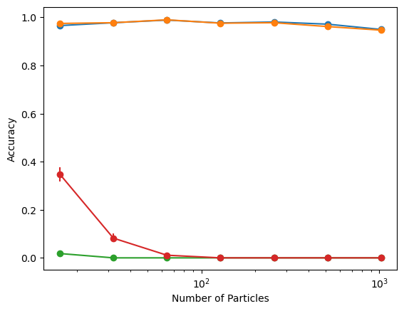
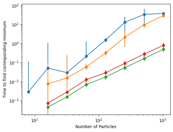
CVODE
Mixed Descent
FIRE
LBFGS
LBFGS
Mixed Descent
CVODE
FIRE
Counting by sampling
\(d\)
$$ N_{buildings} = \frac{D}{\langle\mathcal{d}\rangle} $$
March meeting 2024
By Praharsh Suryadevara


