Gravitational Lensing and the Most Powerful Explosions in the Space
Prajakta Mane
MS19054
IDC451: Seminar Delivery
1
Topic of the Work
2
Gravitational Lensing
3
Why Lensed Type Ia Supernovae
4
Science Steps and Results
Outline of the Presentation
1
Topic of the Work
Outline of the Presentation
- Vera Rubin observatory: Legacy Survey of Space and Time (LSST) Conduct a deep survey of sky for ten years to image about 20000 sq deg of sky in the optical wavelength every week.
- Construct a pipeline to analyze the LSST data to identify the lensed Type Ia supernovae from the data within the LSST stack framework and to analyze the pipeline for its efficiency.
Topic of Work
Source: https://www.lsst.org/about
1
Topic of the Work
2
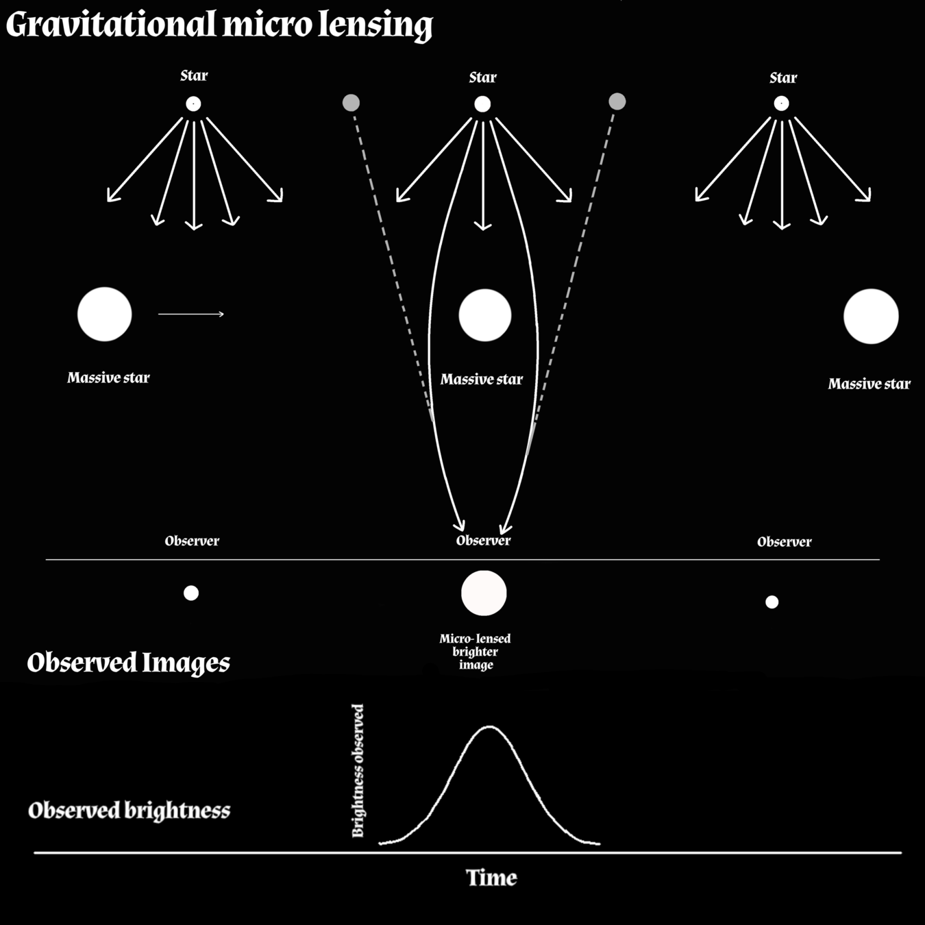
Gravitational Lensing
Outline of the Presentation
-
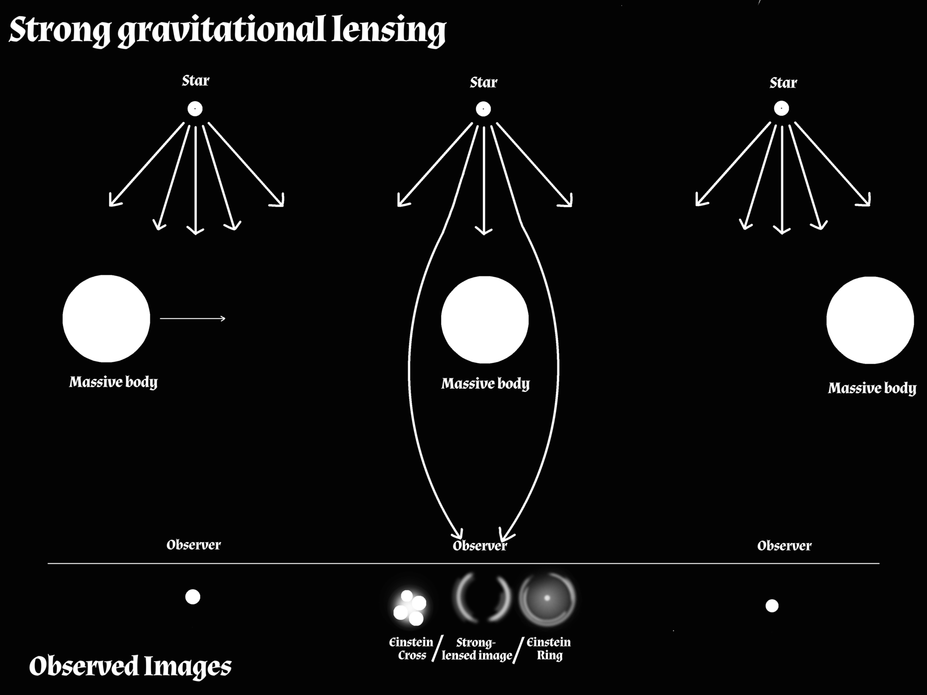
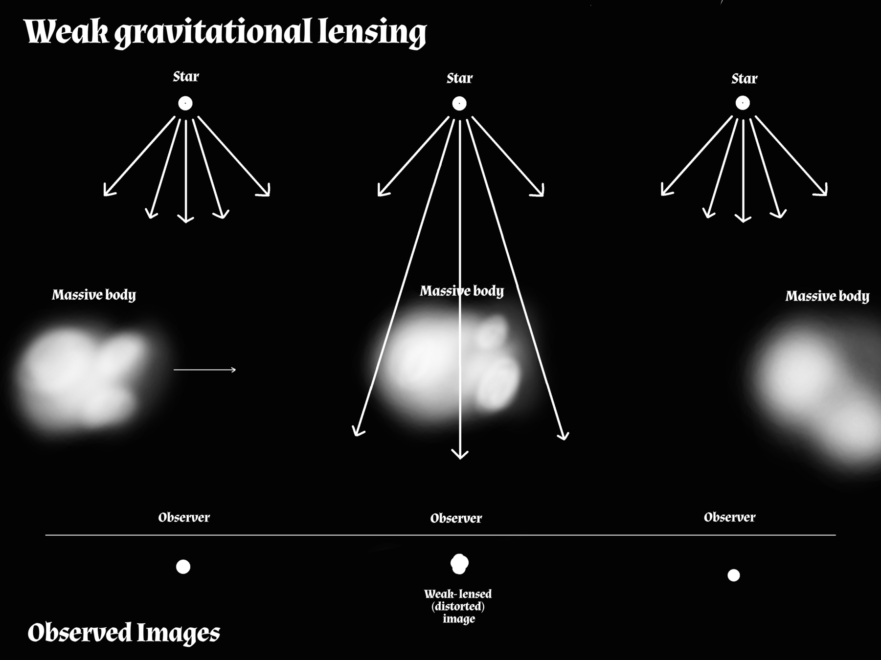
Bending of light due to the gravitational field of massive objects.
-
Different forms
-
Strong gravitational lensing
-
Weak gravitational lensing
-
Microlensing
-
Gravitational Lensing
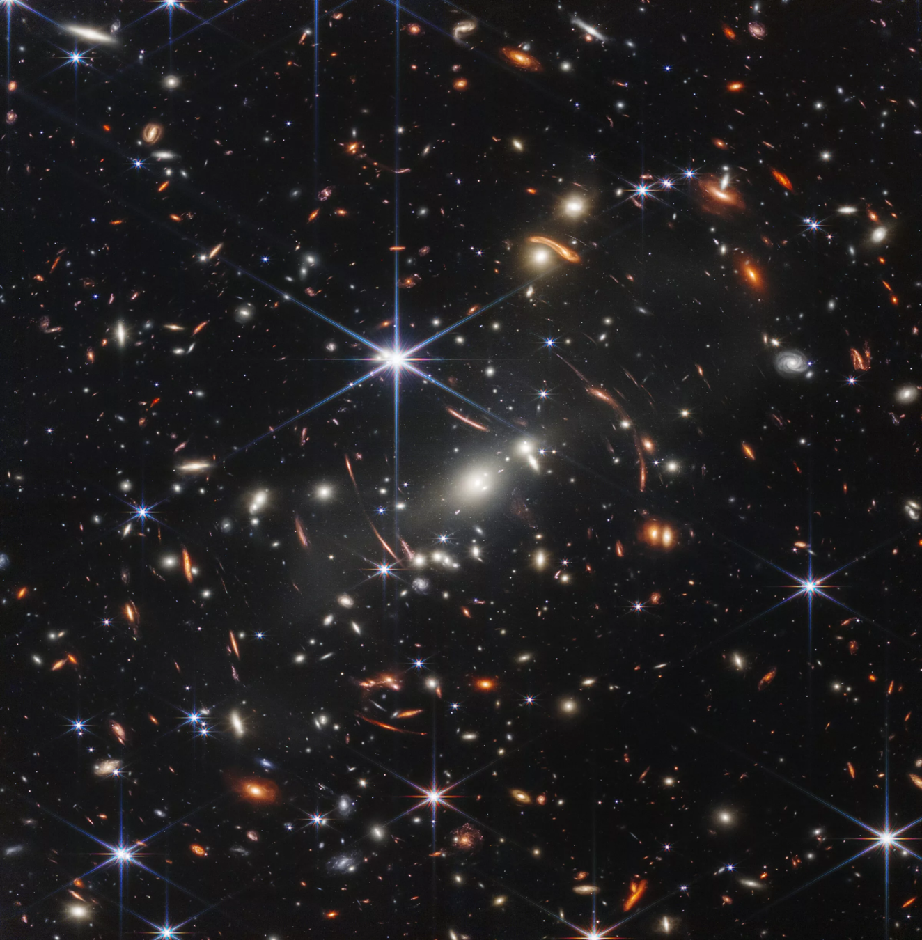
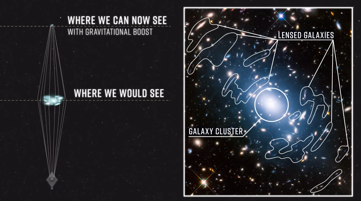
JWST's First Deep Field Image
The Lensing Theory
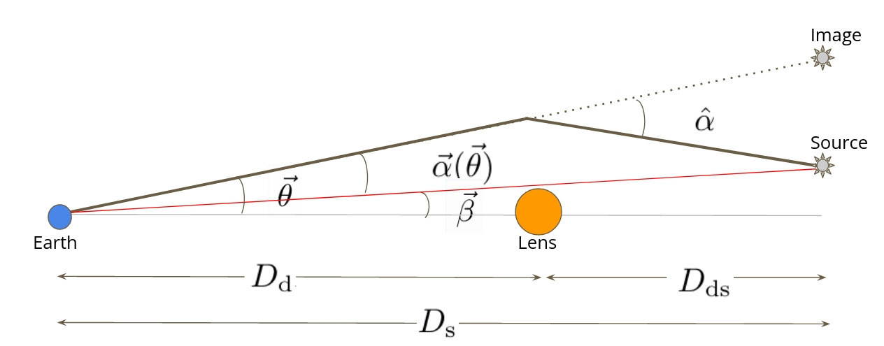
\boldsymbol{\beta} = \boldsymbol{\theta} - \boldsymbol{\alpha}(\boldsymbol{\theta})
Lens Equation
\boldsymbol{\alpha}(\boldsymbol{\theta}) = \frac{D_{ds}}{D_s} \hat{\boldsymbol{\alpha}}(\boldsymbol{\xi}) = \frac{D_{ds}}{D_s} \left[\frac{4G}{c^2}\int D^2_d d^2\boldsymbol{\theta'} \Sigma(D_d\boldsymbol{\theta'}) \frac{D_d (\boldsymbol{\theta}-\boldsymbol{\theta'})}{D^2_d |\boldsymbol{\theta}-\boldsymbol{\theta'}|^2}\right]
The Lensing Theory
\boldsymbol{\beta} = \boldsymbol{\theta} - \boldsymbol{\alpha}(\boldsymbol{\theta})
The Lens Equation
\boldsymbol{\alpha}(\boldsymbol{\theta}) = \frac{D_{ds}}{D_s} \hat{\boldsymbol{\alpha}}(\boldsymbol{\xi}) = \frac{D_{ds}}{D_s} \left[\frac{4G}{c^2}\int D^2_d d^2\boldsymbol{\theta'} \Sigma(D_d\boldsymbol{\theta'}) \frac{D_d (\boldsymbol{\theta}-\boldsymbol{\theta'})}{D^2_d |\boldsymbol{\theta}-\boldsymbol{\theta'}|^2}\right]
Deflection Angle
\boldsymbol{\alpha}(\boldsymbol{\theta}) = \frac{1}{\pi} \left[\int d^2\boldsymbol{\theta'} \kappa(\boldsymbol{\theta}) \frac{\boldsymbol{\theta}-\boldsymbol{\theta'}}{|\boldsymbol{\theta}-\boldsymbol{\theta'}|^2}\right]
\kappa = \frac{\Sigma}{\Sigma_{crit}}
\Sigma_{crit} = \frac{c^2}{4\pi G} \frac{D_s}{D_{ds}D_d}
where
\boldsymbol{\alpha}(\boldsymbol{\theta}) = \boldsymbol{\nabla}_{\boldsymbol{\theta}}\psi
\nabla^2_{\boldsymbol{\theta}}\psi = 2\kappa
Lensing/Deflection Potential and Fermat Potential
\psi(\boldsymbol{\theta}) = \frac{1}{\pi} \int d^2\boldsymbol{\theta'} \kappa(\boldsymbol{\theta'}) ln|\boldsymbol{\theta}-\boldsymbol{\theta'}|
where, lensing/deflection potential is given as,
\tau(\boldsymbol{\theta}, \boldsymbol{\beta}) = \frac{1}{2} (\boldsymbol{\theta} - \boldsymbol{\beta})^2 - \psi(\boldsymbol{\theta})
and Fermat Potential,
The Fermat principle: The physical light rays are those for which the light travel time is stationary.
\therefore \nabla_{\tau}(\boldsymbol{\theta}, \boldsymbol{\beta}) = 0 \implies \boldsymbol{\beta} = \boldsymbol{\theta} - \boldsymbol{\alpha}(\boldsymbol{\theta})
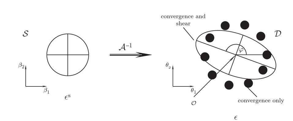
Physical Interpretation
- If the lens equation has more than one solutions for a single value of β then a source at β has images at multiple positions on the sky, leading to multiply lensed source.
- This is satisfied if a mass distribution has κ ≥ 1 i.e., Σ ≥ Σcrit. Σcrit serves as characteristic value for the surface mass density that divides between the strong and the weak lenses.
- This inversion of the lens equation, to obtain the image positions θ from source position β for multiple images, can be carried out analytically only for very simple mass models of the lens. As the number of images θ for a given source β is not known a-priori, a numerical inversion is non-trivial in a general case.
Important Parameters in Lensing
1. Magnification
2. Distortion
3. Time Delay
Magnification and Distortion
-
The magnification of each image is related to the Jacobian of the transformation equation.
M(\boldsymbol{\theta}) = |\mathcal{M}(\boldsymbol{\theta})| = \left|\frac{\partial\boldsymbol{\theta}}{\partial\boldsymbol{\beta}}\right|_{\boldsymbol{\theta}}
\mathcal{M}^{-1}(\boldsymbol{\theta}) = \mathcal{A}(\boldsymbol{\theta})= \left( {\begin{array}{cc}
1-\kappa-\gamma_1 & -\gamma_2 \\
-\gamma_2 & 1-\kappa+\gamma_1 \\
\end{array} } \right)
\gamma_1 = \frac{1}{2}(\psi_{11}-\psi_{22}), \gamma_2 = \psi_{12},\kappa = \frac{1}{2}(\psi_{11}+\psi_{22})
\mathcal{A}(\boldsymbol{\theta}) = \left( {\begin{array}{cc}
1-\kappa & 0 \\
0 & 1-\kappa \\
\end{array} } \right) + \left( {\begin{array}{cc}
-\gamma_1 & -\gamma_2 \\
-\gamma_2 & \gamma_1 \\
\end{array} } \right)
\mu = \det \mathcal{M} = \frac{1}{\det \mathcal{A}} = \frac{1}{(1-\kappa)^2 - |\gamma|^2}
where the magnification matrix is given as,
where the magnification matrix can also be written as,
combination of the symmetric magnification and the sheer
-
The magnification of each image is related to the Jacobian of the transformation equation.
µ = fluxes observed from image/fluxes observed from unlensed source
Magnification and Distortion
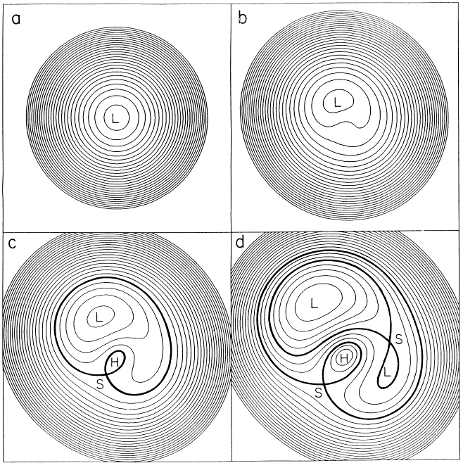
Predicting Multiplicity
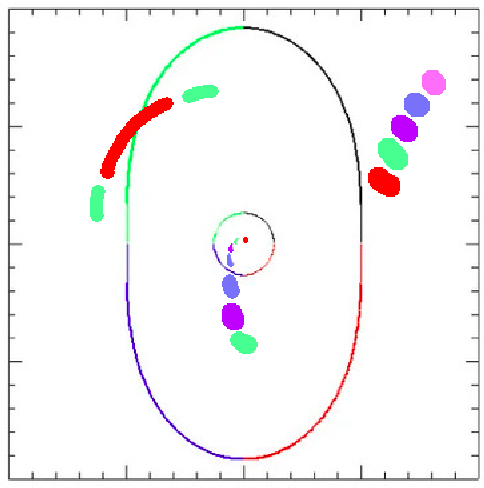
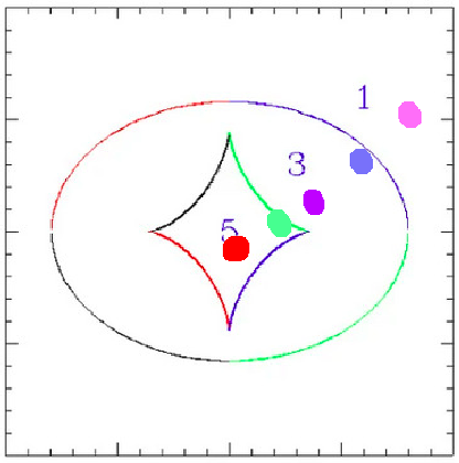
Critical Curves in image plane
Extended, elliptical lens
Joachim Wambsganss, 1998 + Narayan and Bartelmann, 1998
Caustics in source plane
\det \mathcal{A}(\boldsymbol{\theta})= 0
curves
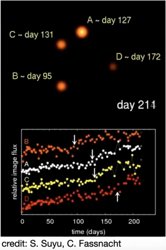
- When the source position crosses a caustic, a pair of images is either created or destroyed near the corresponding critical curve on the lens plane, depending on the direction of crossing.
- The inner side of a caustic produces a pair of images with very high and nearly equal magnification on either side of the critical curve, in addition to any other images.
- The magnification changes sign at the critical curve.
\nabla_{\tau}(\boldsymbol{\theta}, \boldsymbol{\beta}) = 0
Based on the eigenvalues of the Jacobian A, the lensed images can be divided into three types
contours
Blandford and Narayan, 1986
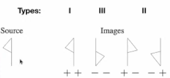
- type I: forms at the minimum of τ, both the eigenvalues positive
- type II: forms at the saddle point of τ, a set of differently signed eigenvalues
- type III: forms at the maximum of the τ, both the eigenvalues negative.
- The source flips its sign in the direction of the eigenvalues in the lens plane.
Time Delay
Two components
1. Geometrical Time Delay: the individual light rays get deflected at different angles, their geometrical lengths are different giving rise to the geometrical time delay.
2. Gravitational Time Delay: light rays propagate through a gravitational potential which retards them, resulting in the gravitational time delay.
Total time delay = geometrical time delay + gravitational time delay
\Delta t= \frac{1+z}{2c} (\boldsymbol{\theta} - \boldsymbol{\beta})^2 \frac{D_d D_s}{D_{ds}} + \frac{1+z}{c} \frac{D_d D_s}{D_{ds}} \psi(\boldsymbol{\theta}) = \frac{D_d D_s}{cD_{ds}}(1+z)\Delta\tau
Outline of the Presentation
- A supernova is a transient astronomical event that occurs during the last evolutionary stages of a massive star or when a white dwarf is triggered into runaway nuclear fusion.
- Is classified according to the light curves and the absorption lines of different chemical elements that appear in the spectra.
- Type Ia supernovae occur in binary systems in which one of the stars is a white dwarf.
- Have the light curves with a sharp maximum and gradual decline, producing a fairly consistent peak luminosity because of the fixed critical mass at which a white dwarf will explode.
- Generally occur in all types of galaxies.
Supernova Type Ia
Why Lensed Type Ia Supernovae
- Standard Candles: Type Ia supernovae are the most useful, precise, and mature tools for determining astronomical distances.
- Dark Energy: Dark energy is often characterized by its ratio of pressure to density with the equation of state ω = P /ρc 2 . If a is an arbitrary length scale in the universe, then the density of some components of the universe evolves as ρ = a −3(1+ω) . Normal matter has ω= 0; it dilutes with volume as space expands. Measurement of <ω> or ω(z) for dark energy is obtained by
building a map of the history of the expansion of the universe using SN Ia as standardized candles. - Independent Method to Constrain the value of the Hubble's Parameter:
\Delta t = \frac{D_d D_s}{D_{ds}}(\frac{1+z}{z})\Delta\tau
\frac{D_d D_s}{D_{ds}} \alpha \frac{1}{H_0}
Collaborations like H0LiCoW, COSMOGRAIL, TDCOSMO
Outline of the Presentation
Data
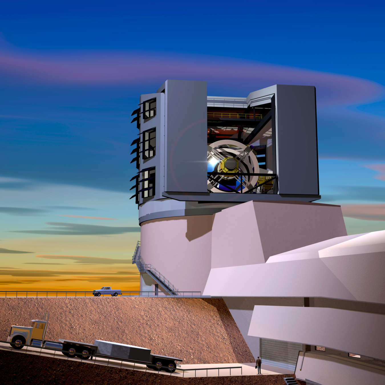
Vera Rubin Observatory and the LSST
- Under construction ion the El Peñón peak of Cerro Pachón in northern Chile.
- Full survey operations expected to begin in October 2024.
- Very wide field of view with a large etendue of 319 m^2 deg^2 .
- LSST, Legacy Survey of Space and Time, over an extended period of 10 years, producing a trillion line database with temporal astrometric and photometric data on 20 billion objects.
Subaru Telescope and Hyper-Suprime Cam
- 8.2-meter optical-infrared telescope at the summit of Maunakea, Hawaii.
- The Hyper Suprime-Cam (HSC), a gigantic mosaic CCD camera attached at the prime focus of Subaru Telescope. Offers an ultra wide field view of the sky.
- Due the similarity between the HSC’s data products and that of the LSST, HSC data is used as the precursor of the LSST for many data analysis pipelines.
Vera Rubin Observatory and the LSST
Outline of the Presentation
Science Steps
Simulating the lensing events
Simulating lensing events for a set of supernovae and generate a catalog of information required for the further step of injection
Science Steps
Simulating the lensing events
Simulating lensing events for a set of supernovae and generate a catalog of information required for the further step of injection
Injecting the information from the catalog produced in step one in a real patch of sky observed by the HSC
(tract 9813) in the LSST Framework. This data, partly real-partly simulated, will be processed further in the LSST Stack.
Injection of simulated information in a real patch of sky
Recovery of the injected information
Subtracting the output image (science image) of the real sky with the injected lensed supernovae from the reference image containing only the real information of the same tract. Further analysis and tests will be performed on the recovered image to determine the efficiency of the the analysis pipeline. The pipeline will be
tweaked, if required, to get better results.
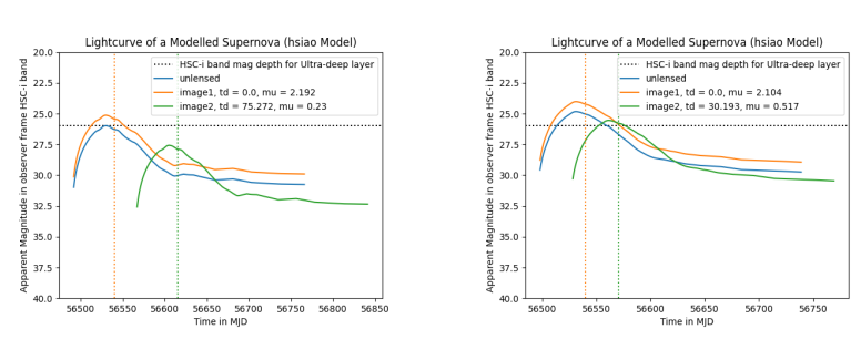
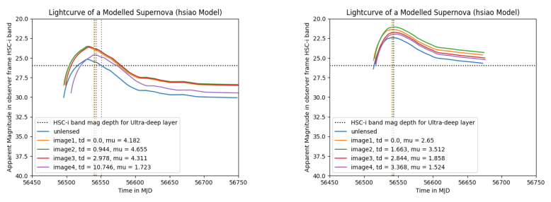
Results
Simulating the lensing events
Light curves of some simulated supernova. X-axis is time in Modified Julian Dates(MJDs) and Y-axis is the apparent magnitude of the source and its lensed images in observer frame HSC-i bandpass. The vertical lines show the t0 parameter of the light curves corresponding to each supernova. The horizontal line shows the maximum magnitude observable by the HSC in Ultra-deep level for i band.
Results
Simulating the lensing events
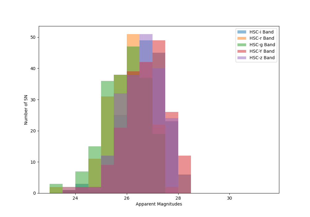
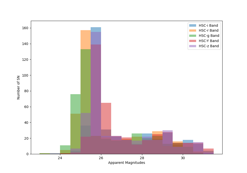
Peak Band Apparent Magnitudes for
Unlensed Supernovae
Peak Band Apparent Magnitudes after Lensing of Supernovae
results
Next two steps are still under Progress.
Future Prospects
We plan continue this project and complete the analysis by performing the science step 2 and 3. Once completed, this pipeline could be used to analyze the upcoming LSST data in order to find the strongly lensed type Ia supernovae.
The type Ia supernovae retrieved with the help of this pipeline from the LSST data could be studied further in the direction of obtaining independent constraints on the value of the Hubble Constant, although this aspect has not been discussed of as of presently.
Thank You
IDC451_Presentation_MS19054
By Prajakta
IDC451_Presentation_MS19054
Presentation made for IDC451: Seminar Delivery course on the topic Gravitational Lensing and the Most Powerful Explosions in the Space


