1.7 Sigmoid Neuron
The building block of Deep Neural Networks
Recap: Six jars
What we saw in the previous chapter?
(c) One Fourth Labs
\( \in \mathbb{R} \)
Classification


loss = \sum_i (y_i-\hat{y_i})^2
Accuracy=\frac{\text{Number of correct predictions}}{\text{Total number of predictions}}
Loss
Model
Data
Task
Evaluation
Learning
Real inputs
Boolean Output
Perceptron Learning Algorithm
Some thoughts on the contest
Just some ramblings!
(c) One Fourth Labs
We should create the binary classification monthly contest such that we can somehow visualize that the data is not linearly separable (don't know how)
We should also be able to visualize why the perceptron model is not fitting
Also give them some insights into what does the loss function indicate and how to make sense of it
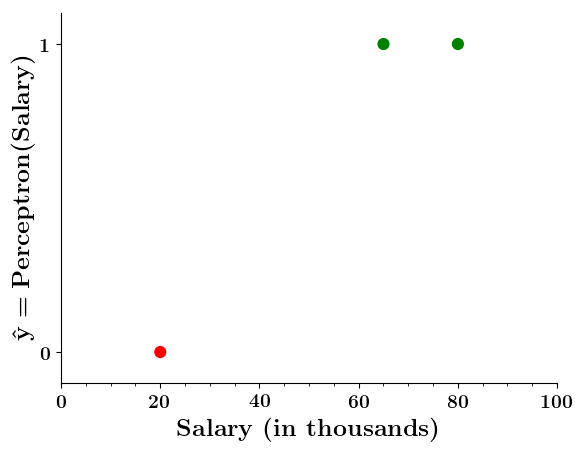
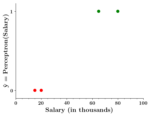
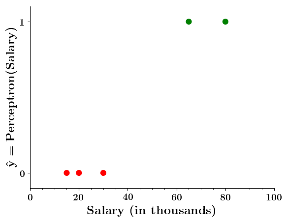
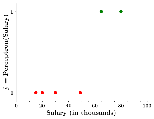
Limitations of Perceptron
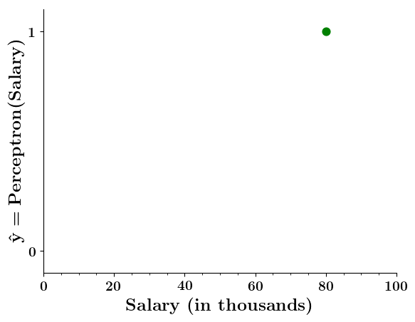
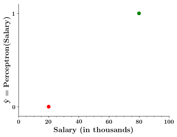
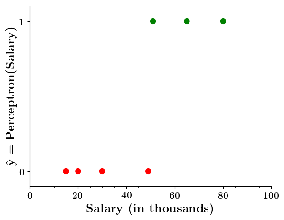
Can we plot the perceptron function ?
(c) One Fourth Labs

Wait a minute!

| Salary ( in thousands) | Can buy a car? |
|---|---|
| 80 | 1 |
| 20 | 0 |
| 65 | 1 |
| 15 | 0 |
| 30 | 0 |
| 49 | 0 |
| 51 | 1 |
| 87 | 1 |
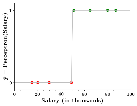
Doesn't the perceptron divide the input space into positive and negative halves ?
y=\sum_{i=1}^n w_i x_i \geq b
\hspace{-1.6cm}\text{Suppose,} \\
\mathbb{w_1} = 0.2, \mathbb{b}\ \ = -10

Limitations of Perceptron
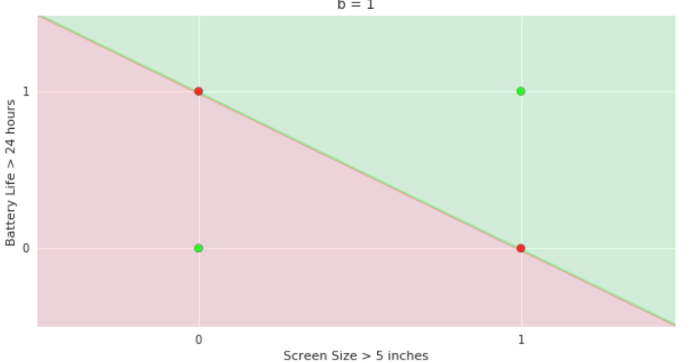
How does the perceptron function look in 2 dimensions?
(c) One Fourth Labs
y=\sum_{i=1}^n w_i x_i \geq b
\text{Suppose,} \\
\mathbb{w_1} = 0.2,\\
\hspace{-0.2cm}\mathbb{w_2} = 0.1 \\
\mathbb{b} = -10.5
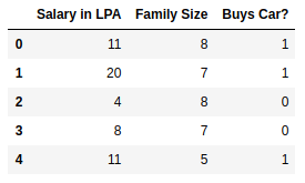
| Salary (in thousands) | Family size | Can buy a car? |
|---|---|---|
| 80 | 2 | 1 |
| 20 | 1 | 0 |
| 65 | 4 | 1 |
| 15 | 7 | 0 |
| 30 | 6 | 0 |
| 49 | 3 | 0 |
| 51 | 4 | 1 |
| 87 | 8 | 1 |
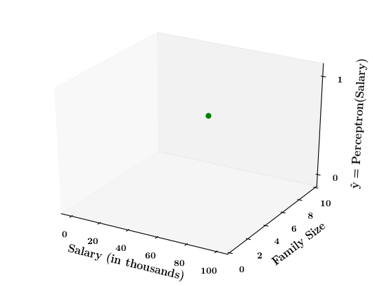
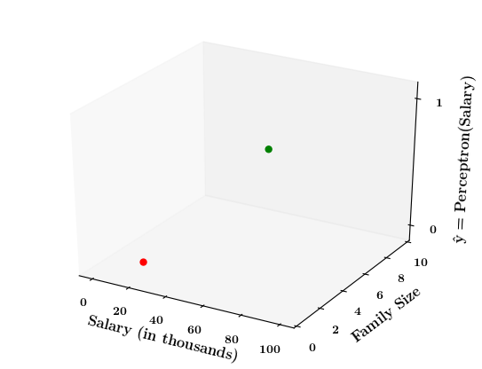
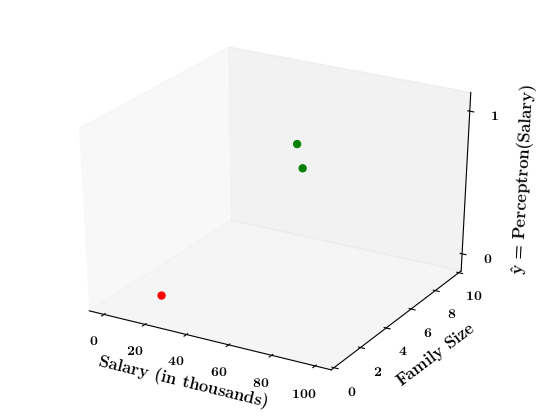
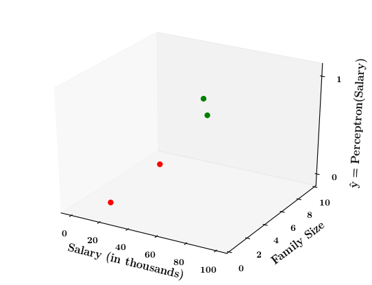
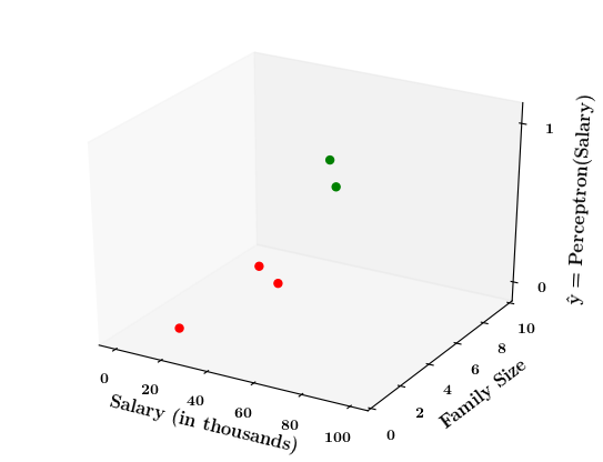
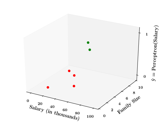
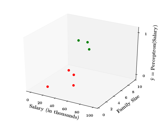
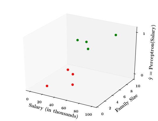

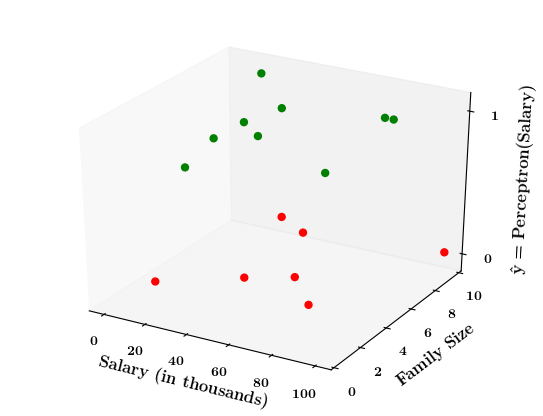
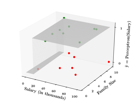
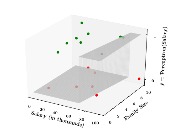
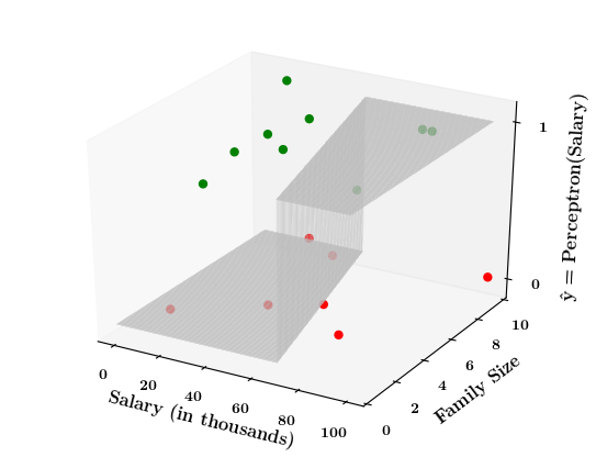
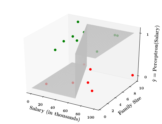
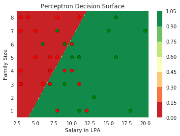
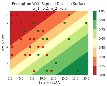
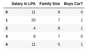
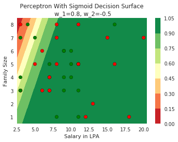
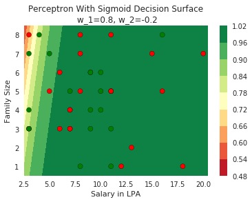
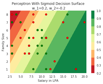
Limitations of Perceptron
What if the data is not linearly separable ?
(c) One Fourth Labs
y=\sum_{i=1}^n w_i x_i \geq b
\text{Suppose,} \\
\mathbb{w_1} = 0.2,\\
\hspace{-0.2cm}\mathbb{w_2} = 0.1 \\
\mathbb{b} = -6
| Salary (in thousands) | Family size | Can buy a car? |
|---|---|---|
| 81 | 8 | 1 |
| 37 | 9 | 0 |
| 34 | 5 | 1 |
| ... | ... | ... |
| 40 | 4 | 0 |
| 100 | 10 | 0 |
| 10 | 10 | 1 |
| 85 | 8 | 1 |
\text{Suppose,} \\
\mathbb{w_1} = 0.2,\\
\hspace{-0.2cm}\mathbb{w_2} = 0.1 \\
\mathbb{b} = -3
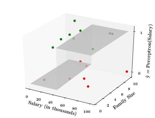
\text{Suppose,} \\
\mathbb{w_1} = 0.2,\\
\hspace{-0.2cm}\mathbb{w_2} = -0.3 \\
\mathbb{b} = -14
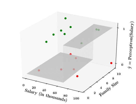
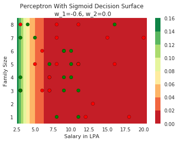
\text{Suppose,} \\
\mathbb{w_1} = 0.2,\\
\hspace{-0.2cm}\mathbb{w_2} = -0.5 \\
\mathbb{b} = -14
\text{Suppose,} \\
\mathbb{w_1} = 0.2,\\
\hspace{-0.2cm}\mathbb{w_2} = 0.1 \\
\mathbb{b} = -9
\text{Suppose,} \\
\mathbb{w_1} = 0.2,\\
\hspace{-0.2cm}\mathbb{w_2} = 0.1 \\
\mathbb{b} = -14
\text{Suppose,} \\
\mathbb{w_1} = 0.2,\\
\hspace{-0.2cm}\mathbb{w_2} = -0.7 \\
\mathbb{b} = -14
\text{Suppose,} \\
\mathbb{w_1} = 0.2,\\
\hspace{-0.2cm}\mathbb{w_2} = 0.3 \\
\mathbb{b} = -14
\text{Suppose,} \\
\mathbb{w_1} = 0.2,\\
\hspace{-0.2cm}\mathbb{w_2} = 0.7 \\
\mathbb{b} = -14


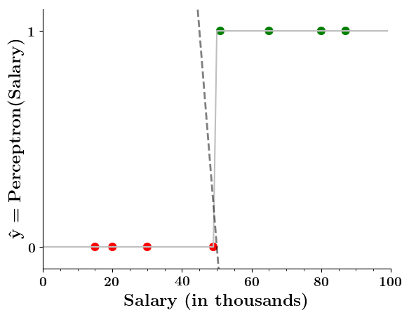
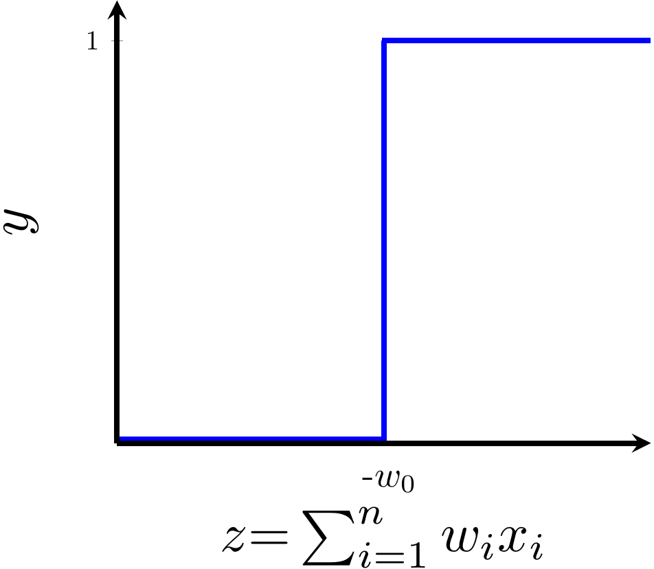
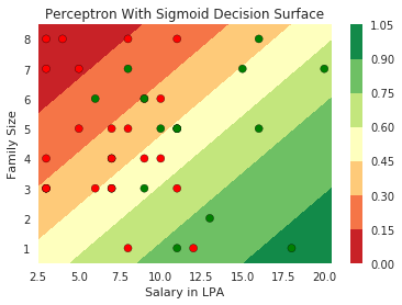
Limitations of Perceptron
Isn't the perceptron model a bit harsh at the boundaries ?
(c) One Fourth Labs
Isn't it a bit odd that a person with 50.1K salary will buy a car but someone with 49.9K will not buy a car ?
| Salary ( in thousands) | Can buy a car? |
|---|---|
| 80 | 1 |
| 20 | 0 |
| 65 | 1 |
| 15 | 0 |
| 30 | 0 |
| 49 | 0 |
| 51 | 1 |
| 87 | 1 |
y=\sum_{i=1}^n w_i x_i \geq b
\text{Suppose,} \\
\mathbb{w_1} = 2,\\
\hspace{-0.2cm}\mathbb{b}\ \ = 1

(c) One Fourth Labs
The Road Ahead
What's going to change now ?
(c) One Fourth Labs
\( \{0, 1\} \)
Boolean
Accuracy=\frac{\text{Number of correct predictions}}{\text{Total number of predictions}}
Loss
Model
Data
Task
Evaluation
Learning
Linear
Real inputs
Boolean output
loss = \sum_i max(0,1-y_i*\hat{y_i})
Specific learning algorithm
Harsh at boundaries
Real output
Non-linear
A more generic learning algorithm
Smooth at boundaries
Data and Task
What kind of data and tasks can Perceptron process ?
(c) One Fourth Labs
Data and Task
What kind of data and tasks can Perceptron process ?
(c) One Fourth Labs
Real inputs
| Launch (within 6 months) | 0 | 1 | 1 | 0 | 0 | 1 | 0 | 1 | 1 |
| Weight (g) | 151 | 180 | 160 | 205 | 162 | 182 | 138 | 185 | 170 |
| Screen size (inches) | 5.8 | 6.18 | 5.84 | 6.2 | 5.9 | 6.26 | 4.7 | 6.41 | 5.5 |
| dual sim | 1 | 1 | 0 | 0 | 0 | 1 | 0 | 1 | 0 |
| Internal memory (>= 64 GB, 4GB RAM) | 1 | 1 | 1 | 1 | 1 | 1 | 1 | 1 | 1 |
| NFC | 0 | 1 | 1 | 0 | 1 | 0 | 1 | 1 | 1 |
| Radio | 1 | 0 | 0 | 1 | 1 | 1 | 0 | 0 | 0 |
| Battery(mAh) | 3060 | 3500 | 3060 | 5000 | 3000 | 4000 | 1960 | 3700 | 3260 |
| Price (INR) | 15k | 32k | 25k | 18k | 14k | 12k | 35k | 42k | 44k |
| Like (y) | 1 | 0 | 1 | 0 | 1 | 1 | 0 | 1 | 0 |


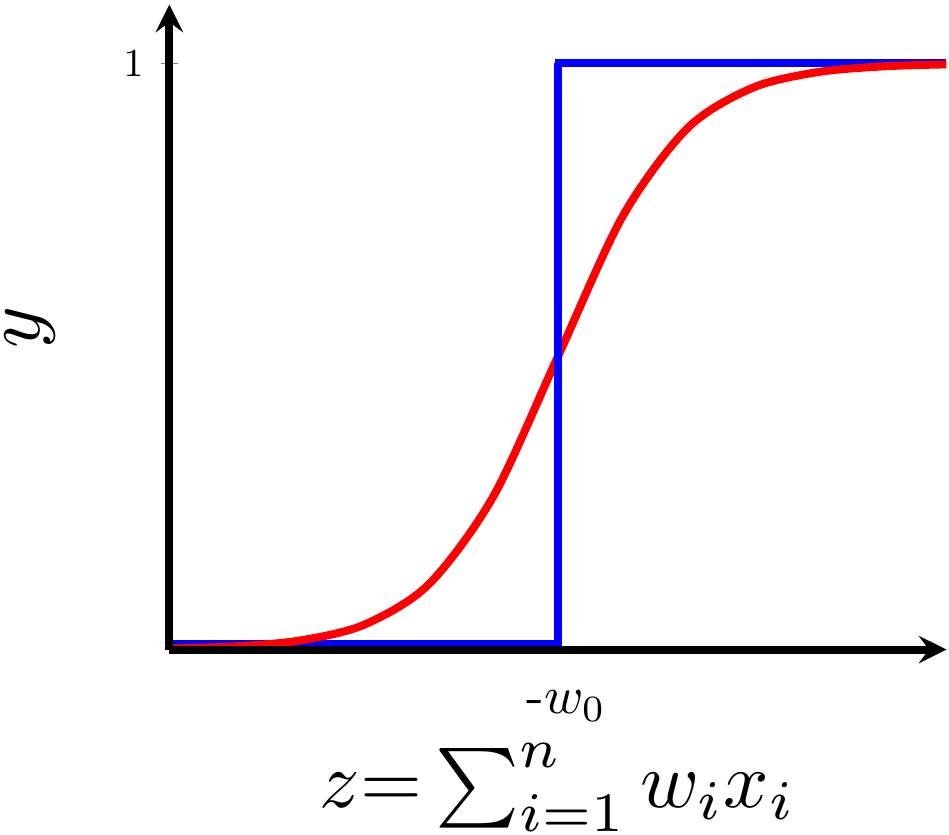
Model
Can we have a smoother (not-so-harsh) function ?
(c) One Fourth Labs
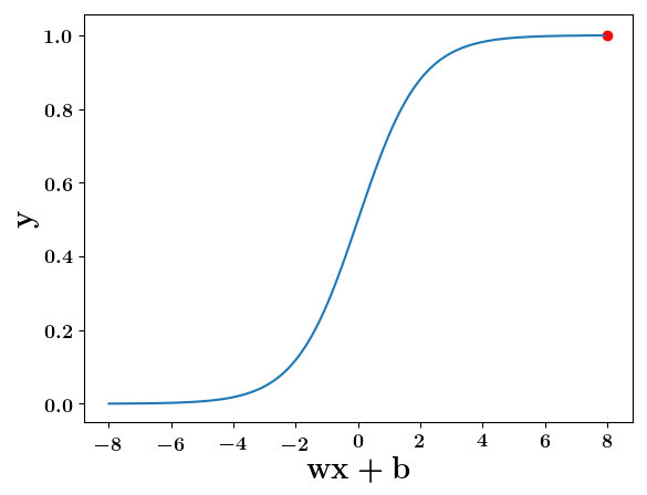
y = \dfrac{1}{1 + e^{-(wx +b)}}
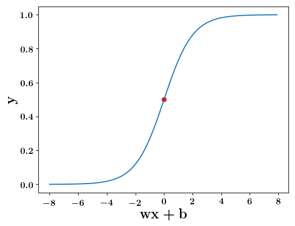
wx+b=0, y=0.5
wx+b=-2, y=0.12
wx+b=2, y=0.88
wx+b=8, y=0.9997
wx+b=-8, y=0.0003


Model
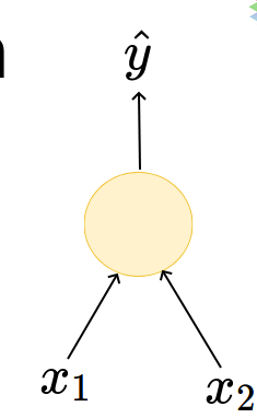
What happens when we have more than 1 input ?
(c) One Fourth Labs
| Launch (within 6 months) | 0 | 1 | 1 | 0 | 0 | 1 | 0 | 1 | 1 |
| Weight (<160g) | 1 | 0 | 1 | 0 | 0 | 0 | 1 | 0 | 0 |
| Screen size (<5.9 in) | 1 | 0 | 1 | 0 | 1 | 0 | 1 | 0 | 1 |
| dual sim | 1 | 1 | 0 | 0 | 0 | 1 | 0 | 1 | 0 |
| Internal memory (>= 64 GB, 4GB RAM) | 1 | 1 | 1 | 1 | 1 | 1 | 1 | 1 | 1 |
| NFC | 0 | 1 | 1 | 0 | 1 | 0 | 1 | 1 | 1 |
| Radio | 1 | 0 | 0 | 1 | 1 | 1 | 0 | 0 | 0 |
| Battery(>3500mAh) | 0 | 0 | 0 | 1 | 0 | 1 | 0 | 1 | 0 |
| Price > 20k | 0 | 1 | 1 | 0 | 0 | 0 | 1 | 1 | 1 |
| Like (y) | 1 | 0 | 1 | 0 | 1 | 1 | 0 | 1 | 0 |
| Prediction | 0 | 0 | 1 | 0 | 0 | 1 | 1 | 1 | 0 |
\hat{y}
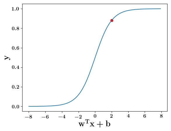
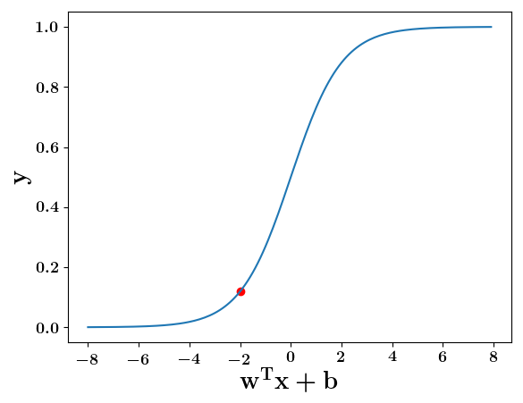
y = \frac{1}{1 + e^{-(\sum_i w_ix_i +b)}}
y = \frac{1}{1 + e^{(-w^Tx+b)}}
w^Tx+b=0, y=0.5
w^Tx+b=2, y=0.88
w^Tx+b=-2, y=0.12

Model
How does this help when the data is not linearly separable ?
(c) One Fourth Labs
Still does not completely solve our problem but we will slowly get there!

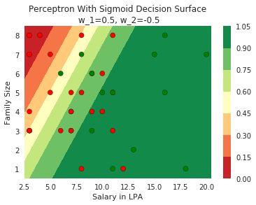


y = \frac{1}{1 + e^{(-w^Tx+b)}}
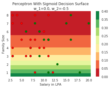
Model
What about extreme non-linearity ?
(c) One Fourth Labs
Still does not completely solve our problem but we will slowly get there with more complex models!


y = \frac{1}{1 + e^{(-w^Tx+b)}}
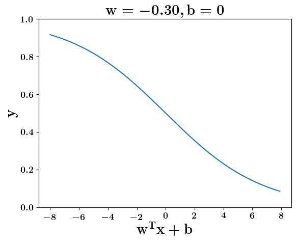
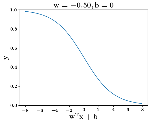
Model
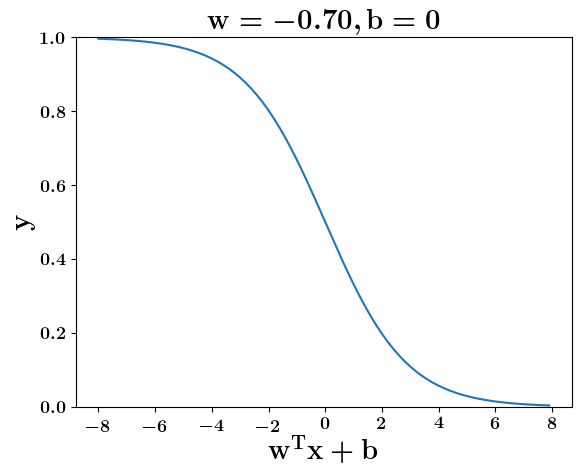
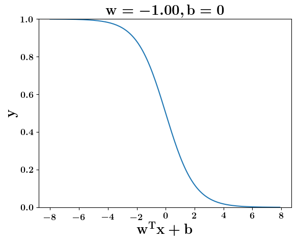
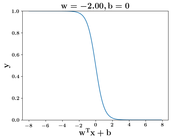
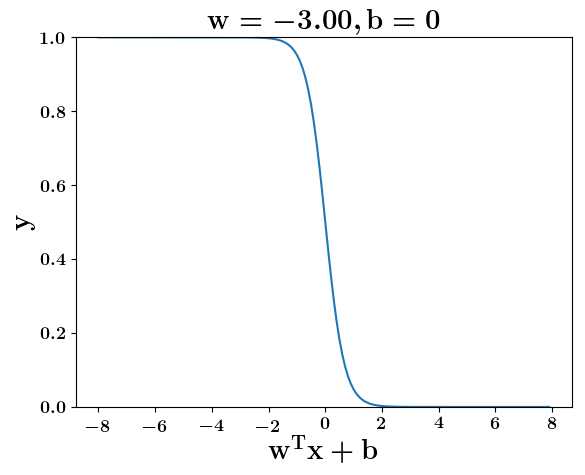
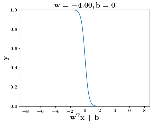
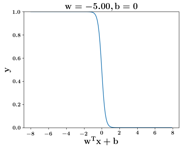
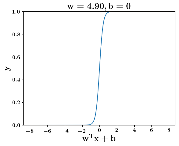
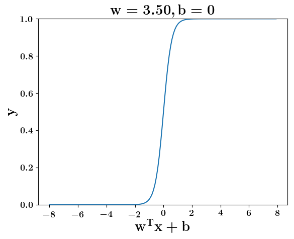
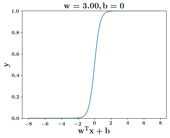
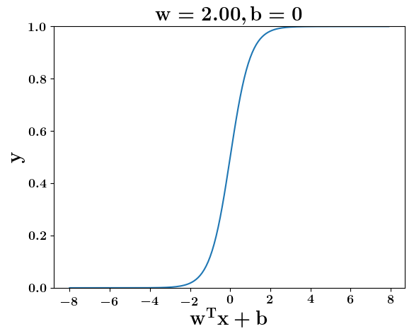
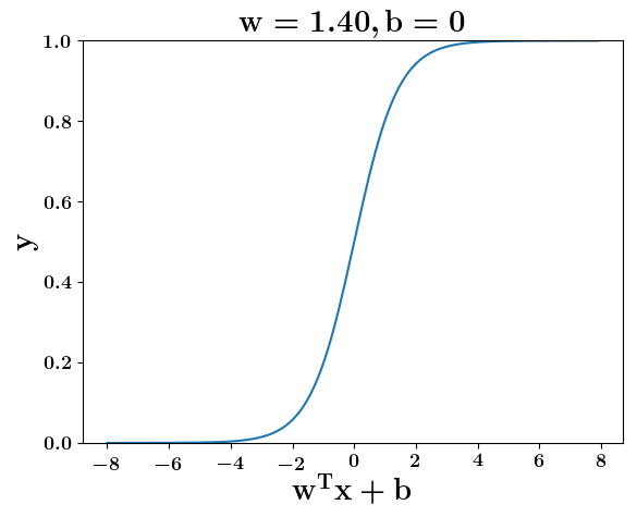
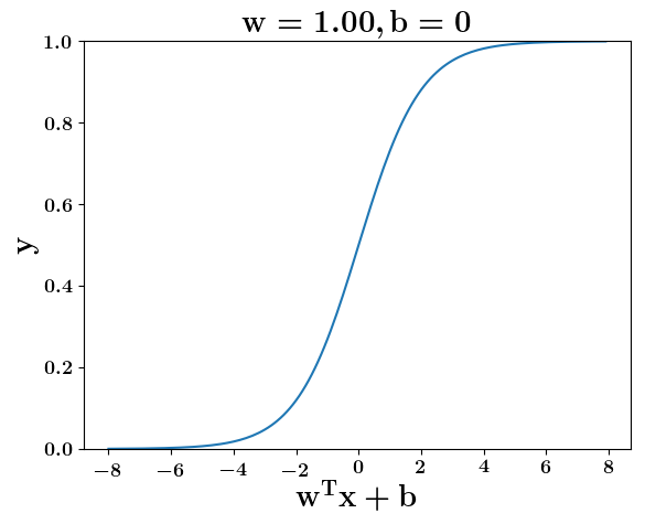
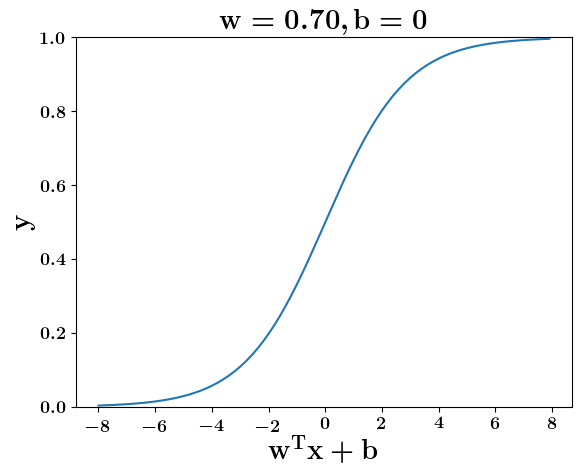
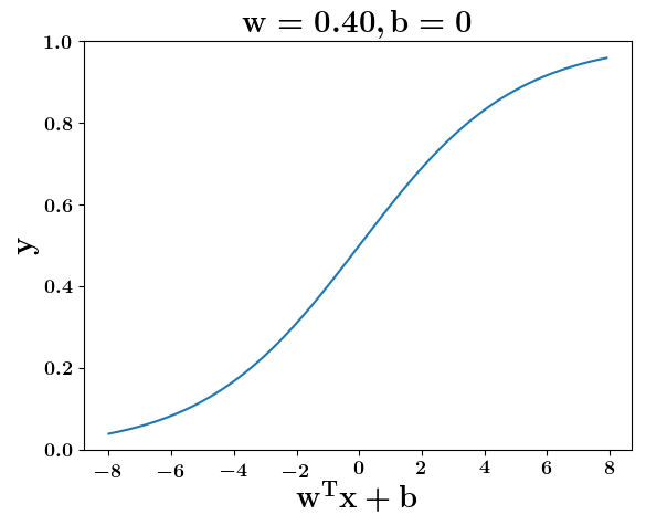
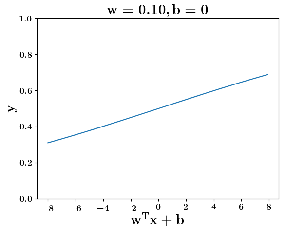
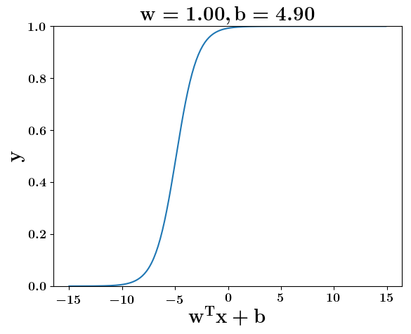
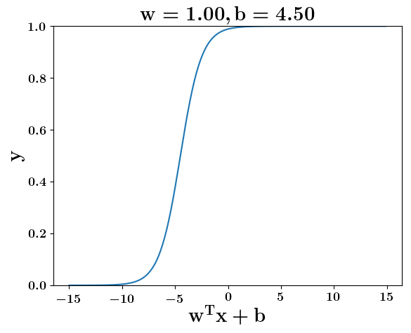
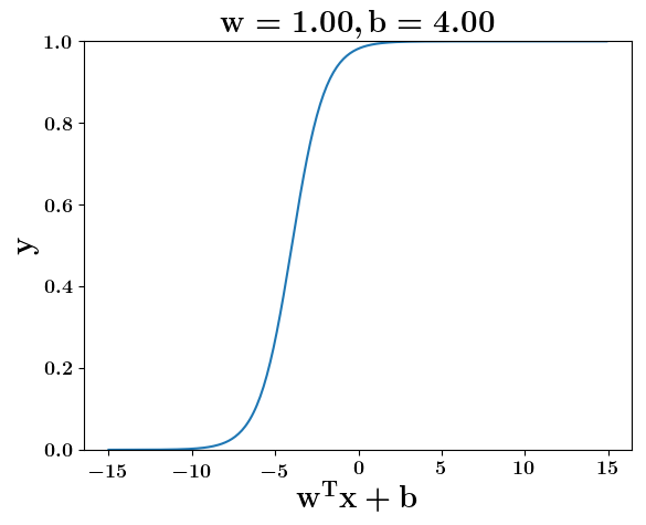
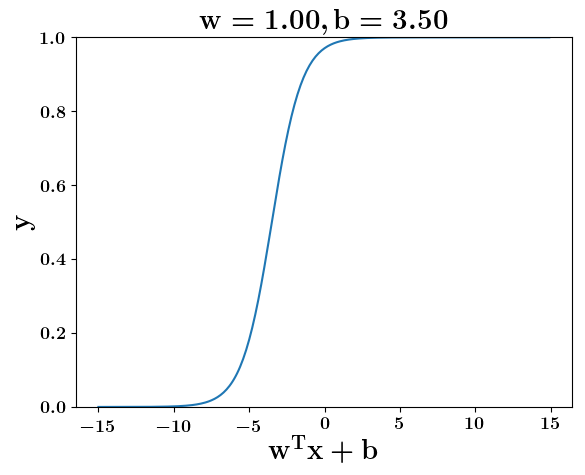
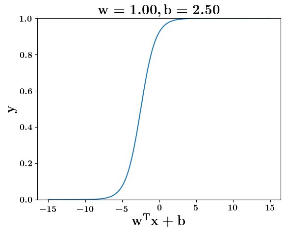
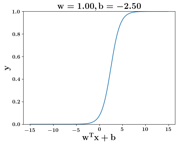
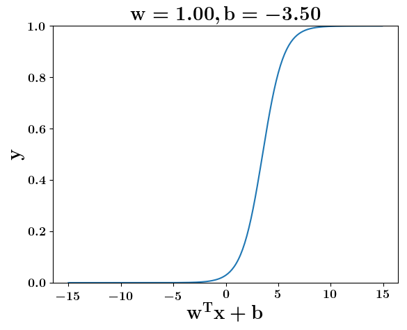
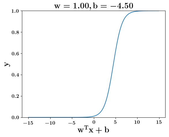
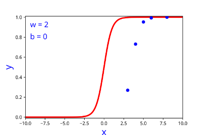
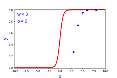
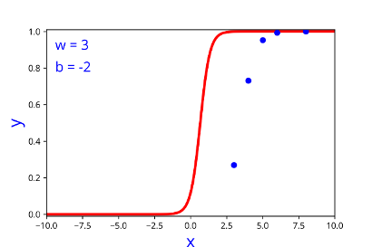
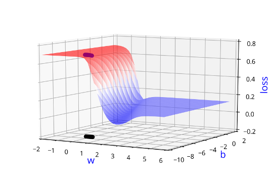
How does the function behave when we change w and b
(c) One Fourth Labs
y =\frac{1}{1+e^{-(wx+b)}}=\frac{1}{2}\\
\implies e^{-(wx+b)} = 1\\
\implies wx+b=0\\
\implies x=-\frac{b}{w}
y = \frac{1}{1 + e^{(-w^Tx+b)}}
At what value of x is the value of sigmoid(X) = 0.5


Loss Function
What is the loss function that you use for this model ?
(c) One Fourth Labs
Can we use loss functions which represent the solution to the problem better? For example, is a bi-quadratic loss a good choice? We will see this later in the course.
| 1 | 1 | 0.5 | 0.6 |
| 2 | 1 | 0.8 | 0.7 |
| 1 | 2 | 0.2 | 0.2 |
| 2 | 2 | 0.9 | 0.5 |
\hat{y}
x_1
x_2
y
Loss=\sum_{i=1}^{4} (y-\hat{y})^2=0.18
\hat{y} = \dfrac{1}{1 + e^{-(wx +b)}}
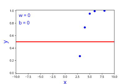
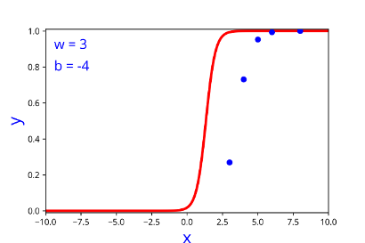
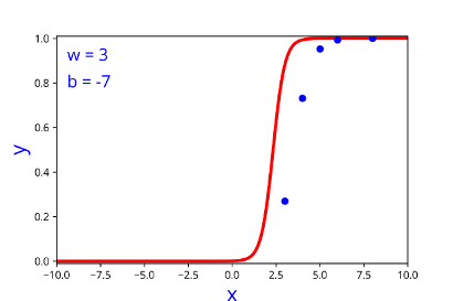
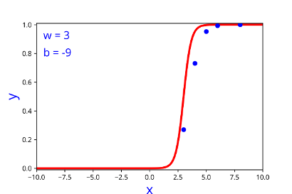
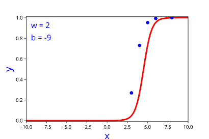
Learning Algorithm
Can we try to estimate w, b using some guess work ?
(c) One Fourth Labs
Initialise
Iterate over data:
till satisfied
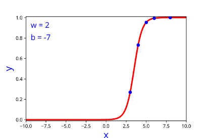
\( h = \frac{1}{1+e^{-(w*x + b)}} \)
| I/P | O/P |
|---|---|
| 2 | 0.047 |
| 3 | 0.268 |
| 4 | 0.73 |
| 5 | 0.952 |
| 8 | 0.999 |
\(w, b \)
\( guess\_and\_update(x_i) \)
| w | b |
|---|---|

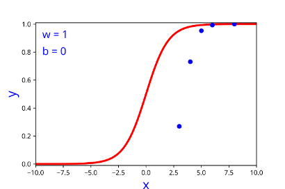
| w | b |
|---|---|
| 1 | 0 |
| w | b |
|---|---|
| 0 | 0 |
| w | b |
|---|---|
| 2 | 0 |
| w | b |
|---|---|
| 3 | -7 |
| w | b |
|---|---|
| 3 | -4 |
| w | b |
|---|---|
| 3 | -2 |
| w | b |
|---|---|
| 3 | 0 |
| w | b |
|---|---|
| 3 | -9 |
| w | b |
|---|---|
| 2 | -9 |
| w | b |
|---|---|
| 2 | -7 |
Learning Algorithm
Can we take a closer look at what we just did ?
(c) One Fourth Labs
Initialise
Iterate over data:
till satisfied
\(w, b \)
\( guess\_and\_update(x_i) \)
| w | b |
|---|---|
| w | b |
|---|---|
| 1 | 0 |
| w | b |
|---|---|
| 0 | 0 |
| w | b |
|---|---|
| 2 | 0 |
| w | b |
|---|---|
| 3 | -7 |
| w | b |
|---|---|
| 3 | -4 |
| w | b |
|---|---|
| 3 | -2 |
| w | b |
|---|---|
| 3 | 0 |
| w | b |
|---|---|
| 3 | -9 |
| w | b |
|---|---|
| 2 | -9 |
\( w = w + \Delta w \\ b = b + \Delta b \)
| w | b |
|---|---|
| 2 | -7 |
1 = 0 + \(\Delta\)1
0 = 0 + \( \Delta\)0
2 = 1 + \(\Delta\)1
0 = 0 + \( \Delta\)0
3 = 2 + \(\Delta\)1
0 = 0 + \( \Delta\)0
3 = 3 + \(\Delta\)0
-2 = 0 + \( \Delta\)-2
3 = 3 + \(\Delta\)0
-4 = -2 + \( \Delta\)-2
3 = 3 + \(\Delta\)0
-7 = -4 + \( \Delta\)-3
3 = 3 + \(\Delta\)0
-9 = -7 + \( \Delta\)-2
2 = 3 + \(\Delta\)-1
-9 = -7 + \( \Delta\)-2
2 = 3 + \(\Delta\)-1
-7 = -9 + \( \Delta\)2
w = 0
b = 0
\( w = w + \Delta w \)
\( b = b + \Delta b \)
\( \Delta w = some\_guess \)
\( \Delta b = some\_guess \)
Learning Algorithm
Can we connect this to the loss function ?
(c) One Fourth Labs
Initialise
Iterate over data:
till satisfied
\(w, b \)
\( guess\_and\_update(x_i) \)
\( w = w + \Delta w \\ b = b + \Delta b \)
1 = 0 + \(\Delta\)1
0 = 0 + \( \Delta\)0
2 = 1 + \(\Delta\)1
0 = 0 + \( \Delta\)0
3 = 2 + \(\Delta\)1
0 = 0 + \( \Delta\)0
3 = 3 + \(\Delta\)0
-2 = 0 + \( \Delta\)-2
3 = 3 + \(\Delta\)0
-4 = -2 + \( \Delta\)-2
3 = 3 + \(\Delta\)0
-7 = -4 + \( \Delta\)-3
3 = 3 + \(\Delta\)0
-9 = -7 + \( \Delta\)-2
2 = 3 + \(\Delta\)-1
-9 = -7 + \( \Delta\)-2
2 = 3 + \(\Delta\)-1
-7 = -9 + \( \Delta\)2
w = 0
b = 0
\( w = w + \Delta w \)
\( b = b + \Delta b \)
| w | b | Loss |
| w | b | Loss |
| 0 | 0 | 0.1609 |
| w | b | Loss |
| 1 | 0 | 0.1064 |
| w | b | Loss |
| 2 | 0 | 0.1210 |
| w | b | Loss |
| 3 | 0 | 0.1217 |
| w | b | Loss |
| 3 | -2 | 0.1215 |
| w | b | Loss |
| 3 | -4 | 0.1198 |
| w | b | Loss |
| 3 | -7 | 0.1081 |
| w | b | Loss |
| 3 | -9 | 0.0209 |
| w | b | Loss |
| 2 | -9 | 0.0636 |
| w | b | Loss |
| 2 | -7 | 0.000 |
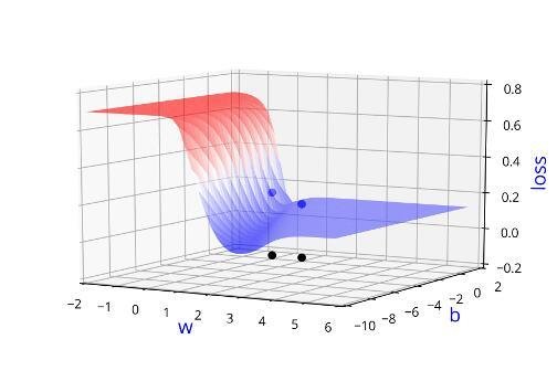
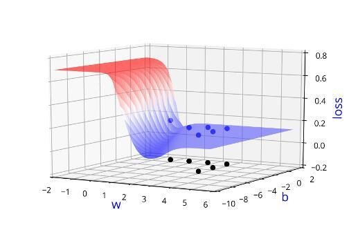
Indeed we were using the loss function to guide us in finding \( \Delta w\) and \(\Delta b\)
Learning Algorithm
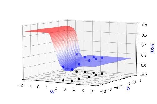
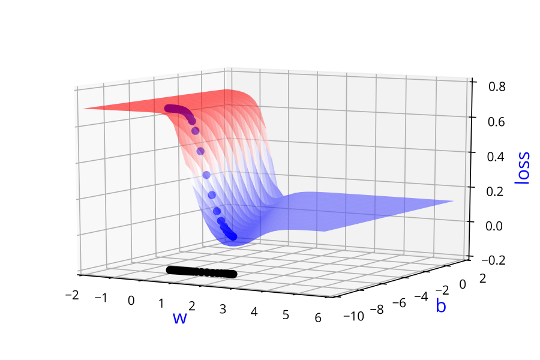
Can we visualise this better ?
(c) One Fourth Labs
Initialise
Iterate over data:
till satisfied
\(w, b \)
\( guess\_and\_update(x_i) \)
\( w = w + \Delta w \\ b = b + \Delta b \)
1 = 0 + \(\Delta\)1
0 = 0 + \( \Delta\)0
2 = 1 + \(\Delta\)1
0 = 0 + \( \Delta\)0
3 = 2 + \(\Delta\)1
0 = 0 + \( \Delta\)0
3 = 3 + \(\Delta\)0
-2 = 0 + \( \Delta\)-2
3 = 3 + \(\Delta\)0
-4 = -2 + \( \Delta\)-2
3 = 3 + \(\Delta\)0
-7 = -4 + \( \Delta\)-3
3 = 3 + \(\Delta\)0
-9 = -7 + \( \Delta\)-2
2 = 3 + \(\Delta\)-1
-9 = -7 + \( \Delta\)-2
2 = 3 + \(\Delta\)-1
-7 = -9 + \( \Delta\)2
w = 0
b = 0
\( w = w + \Delta w \)
\( b = b + \Delta b \)


Learning Algorithm
(c) One Fourth Labs
Initialise
Iterate over data:
till satisfied
\(w, b \)
\( guess\_and\_update(x_i) \)
| w | b |
|---|---|
| w | b |
|---|---|
| 1 | 0 |
| w | b |
|---|---|
| 0 | 0 |
| w | b |
|---|---|
| 2 | 0 |
| w | b |
|---|---|
| 3 | -7 |
| w | b |
|---|---|
| 3 | -4 |
| w | b |
|---|---|
| 3 | -2 |
| w | b |
|---|---|
| 3 | 0 |
| w | b |
|---|---|
| 3 | -9 |
| w | b |
|---|---|
| 2 | -9 |
\( w = w + \Delta w \\ b = b + \Delta b \)
| w | b |
|---|---|
| 2 | -7 |
1 = 0 + \(\Delta\)1
0 = 0 + \( \Delta\)0
2 = 1 + \(\Delta\)1
0 = 0 + \( \Delta\)0
3 = 2 + \(\Delta\)1
0 = 0 + \( \Delta\)0
3 = 3 + \(\Delta\)0
-2 = 0 + \( \Delta\)-2
3 = 3 + \(\Delta\)0
-4 = -2 + \( \Delta\)-2
3 = 3 + \(\Delta\)0
-7 = -4 + \( \Delta\)-3
3 = 3 + \(\Delta\)0
-9 = -7 + \( \Delta\)-2
2 = 3 + \(\Delta\)-1
-9 = -7 + \( \Delta\)-2
2 = 3 + \(\Delta\)-1
-7 = -9 + \( \Delta\)2
w = 0
b = 0
\( w = w + \Delta w \)
\( b = b + \Delta b \)
\( \Delta w = some\_guess \)
\( \Delta b = some\_guess \)
"Instead of guessing \( \Delta w\) and \(\Delta b\), we need a principled way of changing w and b based on the loss function"
What is our aim now ?
Learning Algorithm
Can we formulate this more mathematically ?
(c) One Fourth Labs
\(\theta = [w, b] \)
\(\Delta \theta = [\Delta w, \Delta b] \)
\( \theta_{new} = \theta + \eta . \Delta \theta \)
\(\theta\)
\(\Delta \theta\)
\( \eta . \Delta \theta \)
\( \theta_{new}\)
Instead of guessing \(\Delta w\) and\( \Delta\) b, we need a principled way of changing w and b based on the loss function
Learning Algorithm
Can we get the answer from some basic mathematics ?
(c) One Fourth Labs
\( \because \theta = [w, b] \)
\(w \rightarrow w + \eta \Delta w \)
\(b \rightarrow b + \eta \Delta b \)
\(\mathscr{L} (w) < \mathscr{L}(w +\eta \Delta w)\)
\( \mathscr{L} (b) < \mathscr{L}(b +\eta \Delta b)\)
\(\mathscr{L} ( \theta) < \mathscr{L}( \theta + \eta \Delta \theta)\)
\( f(x + \Delta x) = f(x) + f'(x)\Delta x + \frac{1}{2!}f''(x)\Delta x^2 + \frac{1}{3!}f'''(x)\Delta x^3 + \cdots \)
Taylor Series
\(\mathscr{L} (w,b) < \mathscr{L}(w +\eta \Delta w, b + \eta\Delta b )\)
\( \mathscr{L}(\theta + \Delta \theta) = \mathscr{L}(\theta) + \mathscr{L}'(\theta)\Delta \theta + \frac{1}{2!}\mathscr{L}''(\theta)\Delta \theta^2 + \frac{1}{3!}\mathscr{L}'''(\theta)\Delta \theta^3 + \cdots \)
Learning Algorithm
How does Taylor series help us to arrive at the answer ?
(c) One Fourth Labs
\(\mathscr{L}(\theta+\eta u) = \mathscr{L}(\theta) + \eta*u^T \nabla_{\theta} \mathscr{L}(\theta) + \frac{\eta^2}{2!}*u^T \nabla^2 \mathscr{L} (\theta)u + \frac{\eta^3}{3!}*....+ \frac{\eta^4}{4!}*...\)
\(= \mathscr{L}(\theta)+ \eta*u^T \nabla_{\theta}\mathscr{L}(\theta) [\eta is typically small, so \eta^2, \eta^3, ... \rightarrow 0]\)
Note that the move \( \eta u \) would be favorable only if,
\( \mathscr{L}(\theta+\eta u) - \mathscr{L}(\theta) < 0\) [ i.e. if the new loss is less than the previous loss]
This implies,
\( u^T \nabla_{\theta} \mathscr{L}(\theta) < 0 \)
For ease of notation,
let \( \Delta\theta = u\),
Then from Taylor series, we have,
Learning Algorithm
How does Taylor series help us to arrive at the answer ?
(c) One Fourth Labs
Okay, so we have,
\( u^T \nabla_{\theta} \mathscr{L}(\theta) < 0 \)
But, what is the range of \(u^T \nabla_{\theta}\mathscr{L}(\theta) \) ?
Let \(\beta\) be the angle between \(u\) and \(\nabla_{\theta}\mathscr{L}(\theta)\), then we know that,
\(-1 \leq cos(\beta) = \frac{u^T \nabla_{\theta}\mathscr{L}(\theta)}{||u||*||\nabla_{\theta}\mathscr{L}(\theta)||} \leq 1\)
multiply throughout by k = \( ||u||*||\nabla_{\theta}\mathscr{L}(\theta)||\)
\( -k \leq k*cos(\beta) = u^T \nabla_{\theta}\mathscr{L}(\theta) \leq k \)
Thus, \( \mathscr{L}(\theta + \eta u) - \mathscr{L}(\theta) = u^T \nabla_{\theta}\mathscr{L}(\theta) = k*\cos \beta \) will be most negative
when \(\cos(\beta)\) = -1 i.e., when \(\beta\) is 180\(\degree \)
Learning Algorithm
How does Taylor series help us to arrive at the answer ?
(c) One Fourth Labs
Gradient Descent Rule,
- The direction \(u\) that we intend to move in should be at \(180\degree\) w.r.t. the gradient.
- In other words, move in a direction opposite to the gradient.
Parameter Update Rule
\(w_{t+1} = w_{t} - \eta \Delta w_{t} \)
\(b_{t+1} = b_{t} - \eta \Delta b_{t} \)
\( where \Delta w_{t} =\frac{\partial \mathscr{L}(w, b)}{\partial w}_{at w = w_t, b= b_t}, \Delta b_{t} = \frac{\partial \mathscr{L}(w,b)}{\partial b}_{at w = w_t, b = b_t}\)
So we now have a more principled way of moving in the w-b plane than our "guesswork'' algorithm
Learning Algorithm
How does the algorithm look like now ?
(c) One Fourth Labs
Initialise
\(w, b \)
Iterate over data:
\(w_{t+1} = w_{t} - \eta \Delta w_{t} \)
till satisfied
How do I compute \( \Delta w\) and\( \Delta b \)?
\(b_{t+1} = b_{t} - \eta \Delta b_{t} \)
Learning Algorithm
How do I compute \(\Delta w \) and \(\Delta b\)
(c) One Fourth Labs
\(\mathscr{L} = \frac{1}{5} \sum_{i = 1}^{i=5}(f(x_i) - y_i)\)
\(\frac{\partial \mathscr{L}}{\partial w} = \frac{\partial}{\partial w}[ \frac{1}{5} \sum_{i = 1}^{i=5}(f(x_i) - y_i)]\)
\(\Delta w = \frac{\partial \mathscr{L}}{\partial w} = \frac{1}{5} \sum_{i = 1}^{i=5}\frac{\partial}{\partial w} (f(x_i) - y_i)\)
Let's consider only one term in this sum,
Learning Algorithm
How do I compute \(\Delta w \) and \(\Delta b\)
(c) One Fourth Labs
\(\nabla w = \frac{\partial}{\partial w}[\frac{1}{2}*(f(x) - y)^2] \)
\(= \frac{1}{2}*[2*(f(x) - y) * \frac{\partial}{\partial w} (f(x) - y)]\)
\(= (f(x) - y) * \frac{\partial}{\partial w}(f(x)) \)
\(= (f(x) - y) * \frac{\partial}{\partial w}\Big(\frac{1}{1 + e^{-(wx + b)}}\Big) \)
\( = \color{red}{(f(x) - y) * f(x)*(1- f(x)) *x}\)
\( \frac{\partial}{\partial w}\Big(\frac{1}{1 + e^{-(wx + b)}}\Big)\)
\( =\frac{-1}{(1 + e^{-(wx + b)})^2}\frac{\partial}{\partial w}(e^{-(wx + b)})) \)
\( =\frac{-1}{(1 + e^{-(wx + b)})^2}*(e^{-(wx + b)})\frac{\partial}{\partial w}(-(wx + b)))\)
\( =\frac{-1}{(1 + e^{-(wx + b)})}*\frac{e^{-(wx + b)}}{(1 + e^{-(wx + b)})} *(-x)\)
\( =\frac{1}{(1 + e^{-(wx + b)})}*\frac{e^{-(wx + b)}}{(1 + e^{-(wx + b)})} *(x)\)
\( =f(x)*(1- f(x))*x \)
Learning Algorithm
How do I compute \(\Delta w \) and \(\Delta b\)
(c) One Fourth Labs
\(\mathscr{L} = \frac{1}{5} \sum_{i = 1}^{i=5}(f(x_i) - y_i)\)
\(\frac{\partial \mathscr{L}}{\partial w} = \frac{\partial}{\partial w}[ \frac{1}{5} \sum_{i = 1}^{i=5}(f(x_i) - y_i)]\)
\(\Delta w = \frac{\partial \mathscr{L}}{\partial w} = \frac{1}{5} \sum_{i = 1}^{i=5}\frac{\partial}{\partial w} (f(x_i) - y_i)\)
Let's consider only one term in this sum,
\(\Delta w=(f(x) - y) * f(x)*(1- f(x)) *x \)
For 5 points,
\(\Delta w=\sum_{i=1}^{i=5} (f(x_i) - y_i) *f(x_i))*(1- f(x_i)) *x_i \)
\(\Delta b=\sum_{i=1}^{i=5} (f(x_i) - y_i) * f(x_i))*(1- f(x_i)) \)
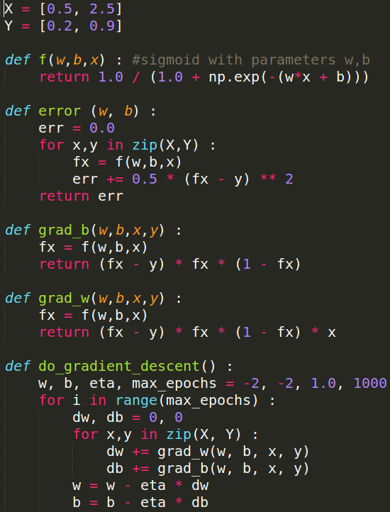
Learning Algorithm
How does the full algorithm look like ?
(c) One Fourth Labs

Learning Algorithm
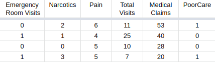
What happens when we have more than 2 parameters ?
(c) One Fourth Labs
\( z = w_1*ER\_visits + w_2*Narcotics + w_3*Pain + w_4*TotalVisits + w_5*MedicalClaims + b \)
\(\hat{y} = \frac{1}{1+e^{-(w_1*x_1 + w_2*x_2 + w_3*x_3 + w_4*x_4 + w_5*x_5 +b)}}\)
\( z = w_1*x_1 + w_2*x_2 + w_3*x_3 + w_4*x_4 + w_5*x_5 + b \)
Initialise
\(w_1, w_2,...,w_5, b \)
Iterate over data:
\(w_1^{t+1} = w_1^{t} - \eta \Delta w_1^{t} \)
till satisfied
\(b_{t+1} = b_{t} - \eta \Delta b_{t} \)
\(w_2^{t+1} = w_2^{t} - \eta \Delta w_2^{t} \)
\(w_5^{t+1} = w_5^{t} - \eta \Delta w_5^{t} \)
\( \vdots \)
\(\Delta w=(f(x) - y) * f(x)*(1- f(x)) *x \)
\(\Delta w_1=(f(x_1,x_2,x_3,x_4,x_5) - y) * f(x_1,x_2,x_3,x_4,x_5)*(1- f(x_1,x_2,x_3,x_4,x_5)) *x_1 \)
\(\hat{y} = \frac{1}{1+e^{-z}}\)
\(\Delta w_1 =(\hat{y} - y) * \hat{y}*(1- \hat{y}) *x_1 \)
Learning Algorithm
How do I compute \(\Delta w \) and \(\Delta b\)
(c) One Fourth Labs
\(\nabla w_1 = \frac{\partial}{\partial w_1}[\frac{1}{2}*(\hat{y} - y)^2] \)
\(= \frac{1}{2}*[2*(\hat{y} - y) * \frac{\partial}{\partial w_1} (\hat{y} - y)]\)
\(= (\hat{y} - y) * \frac{\partial}{\partial w_1}(\hat{y}) \)
\(= (\hat{y} - y) * \frac{\partial}{\partial w_1}\Big(\frac{1}{1 + e^{-(w_1x_1 + w_2x_2 + w_3x_3 + w_4x_4 + w_5x_5 + b)}}\Big) \)
\( = \color{red}{(\hat{y} - y) *\hat{y}*(1- \hat{y}) *x_1}\)
\( \frac{\partial}{\partial w_1}\Big(\frac{1}{1 + e^{-(z)}}\Big)\)
\( =\frac{-1}{(1 + e^{-(z)})^2}\frac{\partial}{\partial w_1}(e^{-(z)})) \)
\( =\frac{-1}{(1 + e^{-(z)})^2}*(e^{-(z)})\frac{\partial}{\partial w_1}(-(z)))\)
\( =\frac{-1}{(1 + e^{-(z)})}*\frac{e^{-(z)}}{(1 + e^{-(z)})} *(-x_1)\)
\( =\frac{1}{(1 + e^{-(z)})}*\frac{e^{-(z)}}{(1 + e^{-(z)})} *(x_1)\)
\( =\hat{y}*(1- \hat{y})*x_1 \)
\( z = w_1*x_1 + w_2*x_2 + w_3*x_3 + w_4*x_4 + w_5*x_5 + b \)
\( \frac{\partial}{\partial w_1}(-z) = - \frac{\partial }{\partial w_1} (w_1*x_1 + w_2*x_2 + w_3*x_3 + w_4*x_4 + w_5*x_5 + b) \)
\( \frac{\partial}{\partial w_1}(-z) = - x_1 \)
Learning Algorithm
How do I compute \(\Delta w \) and \(\Delta b\)
(c) One Fourth Labs
\(\mathscr{L} = \frac{1}{2}(\hat{y} - y)^{2}\)
\(\frac{\partial \mathscr{L}}{\partial w_1} = \frac{\partial}{\partial w_1}(\frac{1}{2} [\hat{y} - y]^2)\)
\(\vdots\)
\(\frac{\partial \mathscr{L}}{\partial w_5} = \frac{\partial}{\partial w_5}(\frac{1}{2} [\hat{y} - y]^2)\)
\(\frac{\partial \mathscr{L}}{\partial w_2} = \frac{\partial}{\partial w_2}(\frac{1}{2} [\hat{y} - y]^2)\)
\(\Delta w_1 =(\hat{y} - y) * \hat{y}*(1- \hat{y}) *x_1 \)
\(\Delta w_2 =(\hat{y} - y) * \hat{y}*(1- \hat{y}) *x_2 \)
\(\Delta w_5 =(\hat{y} - y) * \hat{y}*(1- \hat{y}) *x_5 \)
\(\vdots\)
Learning Algorithm
How do I compute \(\Delta w \) and \(\Delta b\)
(c) One Fourth Labs
\(\begin{bmatrix} \Delta w_1 \\ \Delta w_2 \\ \vdots \\ \Delta w_5 \end{bmatrix} \)
\( \begin{bmatrix} (\hat{y}-y)*\hat{y}*(1-\hat{y})*x_1\\ (\hat{y}-y)*\hat{y}*(1-\hat{y})*x_2 \\ \vdots \\ (\hat{y}-y)*\hat{y}*(1-\hat{y})*x_5\end{bmatrix}\)
\( \Delta w \)
=
=
\( (\hat{y}-y)*\hat{y}*(1-\hat{y}) \begin{bmatrix} x_1 \\ x_2 \\ \vdots \\ x_5 \end{bmatrix} \)
=
Learning Algorithm
How does the full algorithm look like ?
(c) One Fourth Labs


How do you check the performance of the sigmoid model?
(c) One Fourth Labs
Evaluation
| 1 | 0 | 0 | 1 |
| 0.2 | 0.73 | 0.6 | 0.8 |
| 0.2 | 0.7 | 0.8 | 0.9 |
| 0 | 1 | 0 | 0 |
| 1 | 0 | 0 | 0 |
| 0 | 0 | 1 | 0 |
| 1 | 1 | 1 | 0 |
| 0.83 | 0.96 | 0.9 | 0.2 |
| 0.34 | 0.4 | 0.6 | 0.1 |
| 0.17 | 0.56 | 0.3 | 0.4 |
| 0.24 | 0.67 | 0.9 | 0.3 |
Training data
Test data
Accuracy=\frac{\text{Number of correct predictions}}{\text{Total number of predictions}}
= \frac{3}{4} = 75\%
Loss=\sum_{i=1}^{n} (y-\hat{y})^2
y = \frac{1}{1 + e^{(-w^Tx+b)}}
| Launch (within 6 months) | 0 | 1 | 1 | 0 | 0 | 1 | 0 | 1 | 1 |
| Weight | 0.19 | 0.63 | 0.33 | 0.99 | 0.36 | 0.66 | 0.1 | 0.70 | 0.48 |
| Screen size | 0.64 | 0.87 | 0.67 | 0.88 | 0.7 | 0.91 | 0.04 | 0.98 | 0.47 |
| dual sim | 1 | 1 | 0 | 0 | 0 | 1 | 0 | 1 | 0 |
| Internal memory (>= 64 GB, 4GB RAM) | 1 | 1 | 1 | 1 | 1 | 1 | 1 | 1 | 1 |
| NFC | 0 | 1 | 1 | 0 | 1 | 0 | 1 | 1 | 1 |
| Radio | 1 | 0 | 0 | 1 | 1 | 1 | 0 | 0 | 0 |
| Battery | 0.36 | 0.51 | 0.36 | 0.97 | 0.34 | 0.67 | 0 | 0.57 | 0.43 |
| Price | 0.09 | 0.63 | 0.41 | 0.19 | 0.06 | 0 | 0.72 | 0.94 | 1 |
| Like (y) | 0.9 | 0.3 | 0.85 | 0.2 | 0.5 | 0.98 | 0.1 | 0.88 | 0.23 |
Take-aways
What are the new things that we learned in this module ?
(c) One Fourth Labs
Tasks with real inputs and real outputs
Data
Task
Model
Loss
Learning
Evaluation
Loss=
\( w = w + \Delta w \)
\( b = b + \Delta b \)
Accuracy=\frac{\text{Number of correct predictions}}{\text{Total number of predictions}}
\sum_{i=1}^{n} (y-\hat{y})^2
\(w_{t+1} = w_{t} - \eta \Delta w_{t} \)
\(b_{t+1} = b_{t} - \eta \Delta b_{t} \)
\( \in \mathbb{R} \)
Real inputs
OR
Take-aways
Comparison of MP Neuron, perceptron and sigmoid in terms of 6 jars
(c) One Fourth Labs
Still not complex enough to handle non-linear data....
Data
Task
Model
Loss
Learning
Evaluation
\( \{0, 1\} \)
MP neuron
Perceptron
Sigmoid
Real inputs
Real inputs
Binary Classification
Binary Classification
Tasks with real inputs and real outputs
y = \frac{1}{1 + e^{(-w^Tx+b)}}

\hat{y} = 1 \text{ if } \sum_{i=1}^n w_i x_i \geq b
\hat{y} = 0 \text{ otherwise }
\hat{y} = 1 \text{ if } \sum_{i=1}^n x_i \geq b
\hat{y} = 0 \text{ otherwise }
Loss=
\sum_{i=1}^{n} (y-\hat{y})^2
Loss=
\sum_{i=1}^{n} (y-\hat{y})^2
Loss=
\sum_{i=1}^{n} (y-\hat{y})^2

Perceptron Learning Algorithm
Gradient Descent
Accuracy=\frac{\text{Number of correct predictions}}{\text{Total number of predictions}}
Accuracy=\frac{\text{Number of correct predictions}}{\text{Total number of predictions}}
Accuracy=\frac{\text{Number of correct predictions}}{\text{Total number of predictions}}
Copy of Copy of Ameet's Copy of 1.7 Sigmoid Neuron
By preksha nema


