1.9 Multilayered Network of Neurons

Your first Deep Neural Network

Learning Algorithm


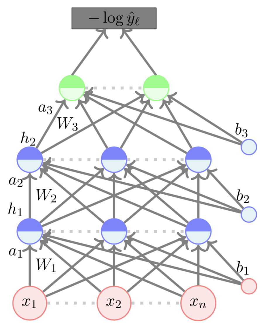
Forward Propogation 

W_2 = \begin{bmatrix} 0.4 & 0.5 & -0.3 \\ -0.1 & -0.4 & -0.5\\ 0.8 & 0.2 & 0.9\\ \end{bmatrix}
b = [\ \ 0\ \ \ 0\ \ 0\ \ ]
y = [\ \ 1 \ \ \ 0\ \ ]
x = [\ \ 2\ \ \ 5 \ \ \ 3 \ \ ]

\(a_1   =   W_1*x + b_1      =   [   -2.2    -0.1         5.3   ]\) 

\(h_1   =   tanh(a_1)   =   [  -0.97        -0.1      0.99   ]\)

\(a_2   =   W_2*h_1 + b_2   =   [   0.41  -0.24    1.24    ]\)

Output :

\(L(\Theta) = -\text{log}\hat{y_l} = 0.43 \)
W_1 = \begin{bmatrix} 0.1 & 0.3 & 0.8\\ -0.3 & -0.2 & 0.5 \\ -0.3 & 0.1 & 0.4 \\ \end{bmatrix}
W_3 = \begin{bmatrix} 0.3 & -0.5\\ 0.1 & 0.2\\ -0.1 & -0.4\\ \end{bmatrix}

\(h_2   =   tanh(a_2)   =   [  0.39        -0.24      0.84   ]\)

\(a_3   =   W_3 * h_2 + b_3   =   [  0.01        -0.58   ]\)

\(\hat{y}   =  softmax(a_3) =   [  0.64        0.36   ]\)

Learning Algorithm


Backward Propogation

W_2 = \begin{bmatrix} 0.4 & 0.5 & -0.3 \\ -0.1 & -0.4 & -0.5\\ 0.8 & 0.2 & 0.9\\ \end{bmatrix}
b = [\ \ 0\ \ \ 0\ \ 0\ \ ]
y = [\ \ 1 \ \ \ 0\ \ ]
x = [\ \ 2\ \ \ 5 \ \ \ 3 \ \ ]

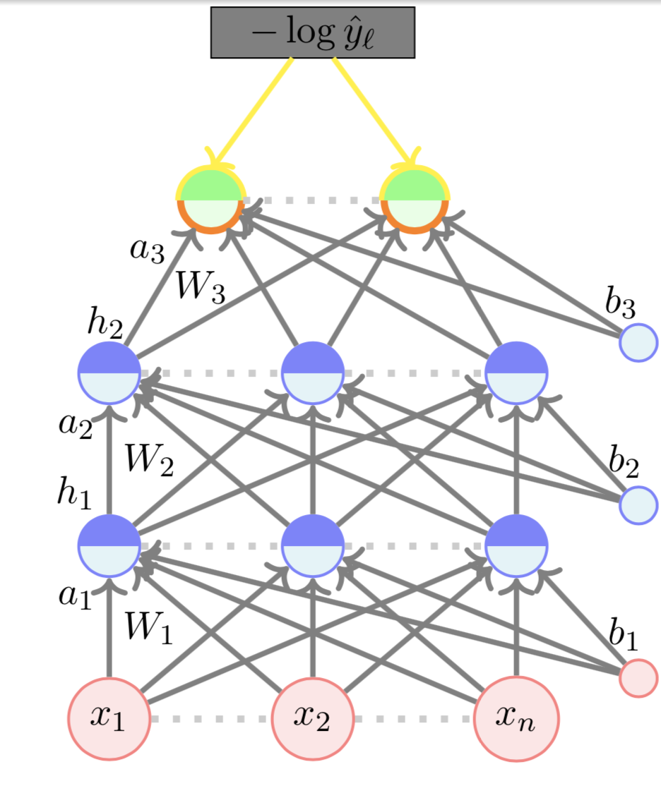
\( \nabla_{a_L} \mathscr{L}(\theta)\) :
W_1 = \begin{bmatrix} 0.1 & 0.3 & 0.8\\ -0.3 & -0.2 & 0.5 \\ -0.3 & 0.1 & 0.4 \\ \end{bmatrix}
W_3 = \begin{bmatrix} 0.3 & -0.5\\ 0.1 & 0.2\\ -0.1 & -0.4\\ \end{bmatrix}
= \begin{bmatrix} \frac{\partial \mathscr{L}{\theta}}{\partial a_{L1}} \\ \\ \frac{\partial \mathscr{L}{\theta}}{\partial a_{L2 }}\\ \end{bmatrix}
= \begin{bmatrix} - (\mathbb{1}_{\ell = 1} - \hat{y}_1)\\ \\ - (\mathbb{1}_{\ell = 2} - \hat{y}_2)\\ \end{bmatrix}
= \begin{bmatrix} - (1 - 0.64)\\ \\ - (0 - 0.36)\\ \end{bmatrix}
= \begin{bmatrix} - 0.36\\ \\ 0.36\\ \end{bmatrix}

Learning Algorithm


Backward Propogation

W_2 = \begin{bmatrix} 0.4 & 0.5 & -0.3 \\ -0.1 & -0.4 & -0.5\\ 0.8 & 0.2 & 0.9\\ \end{bmatrix}
b = [\ \ 0\ \ \ 0\ \ 0\ \ ]
y = [\ \ 1 \ \ \ 0\ \ ]
x = [\ \ 2\ \ \ 5 \ \ \ 3 \ \ ]

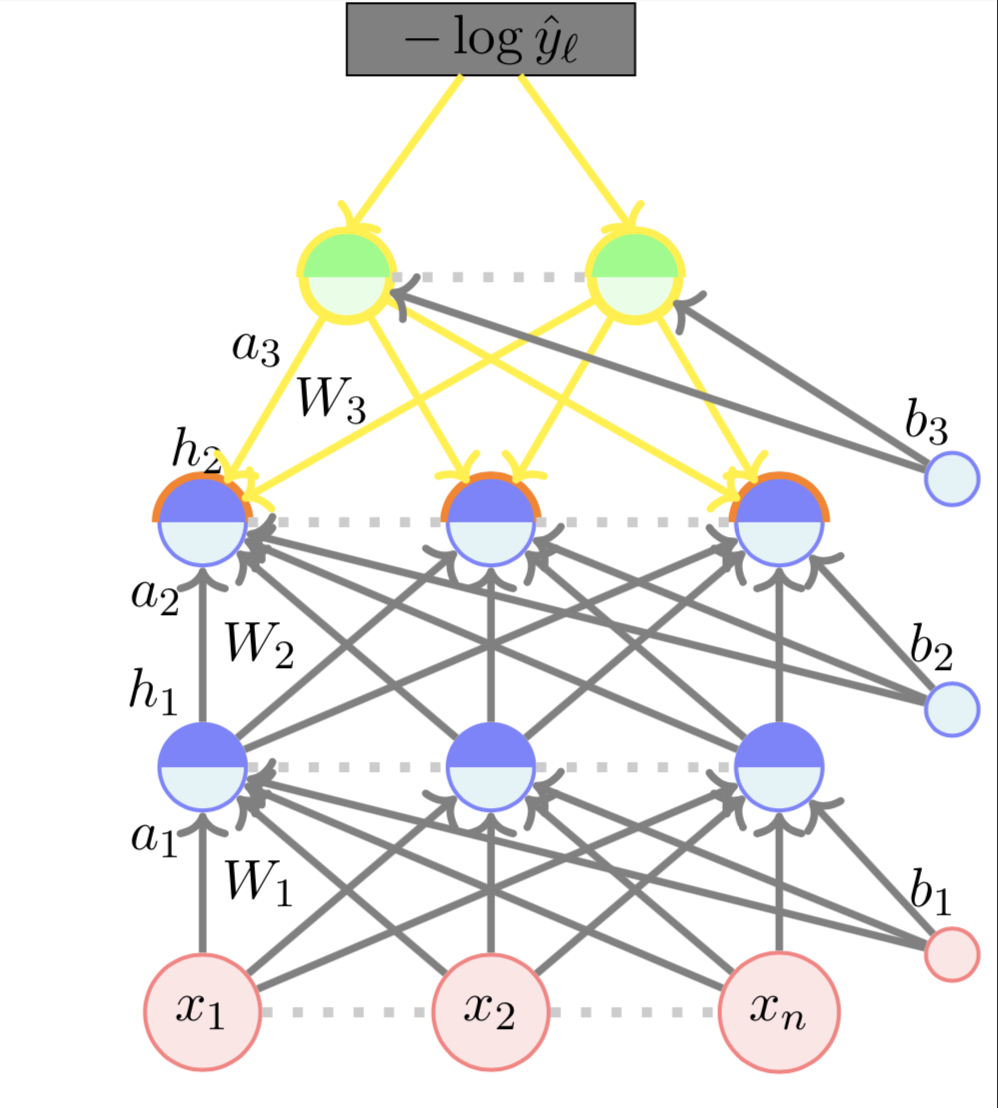
\( \nabla_{h_2} \mathscr{L}(\theta)\) :
W_1 = \begin{bmatrix} 0.1 & 0.3 & 0.8\\ -0.3 & -0.2 & 0.5 \\ -0.3 & 0.1 & 0.4 \\ \end{bmatrix}
W_3 = \begin{bmatrix} 0.3 & -0.5\\ 0.1 & 0.2\\ -0.1 & -0.4\\ \end{bmatrix}
= \begin{bmatrix} \frac{\partial \mathscr{L}{\theta}}{\partial h_{21}} \\ \\ \frac{\partial \mathscr{L}{\theta}}{\partial h_{22 }}\\ \\ \frac{\partial \mathscr{L}{\theta}}{\partial h_{23 }}\\ \end{bmatrix}
= \begin{bmatrix} (W_{2,., 1})^{T} \textcolor{red}{\nabla_{a_{3}} \mathscr{L}({\theta})}\\ \\ (W_{2,., 2})^{T} \textcolor{red}{\nabla_{a_{3}} \mathscr{L}({\theta})}\\ \\ (W_{2,., 3})^{T} \textcolor{red}{\nabla_{a_{3}} \mathscr{L}({\theta})}\\ \end{bmatrix}
= \begin{bmatrix} 0.23\\ \\ - 0.03\\ \\ 0.09 \end{bmatrix}

\( \nabla_{a_3} \mathscr{L}(\theta)\) :

= \begin{bmatrix} \frac{\partial \mathscr{L}{\theta}}{\partial a_{L1}} \\ \\ \frac{\partial \mathscr{L}{\theta}}{\partial a_{L2 }}\\ \end{bmatrix}
= \begin{bmatrix} - 0.36\\ \\ 0.36\\ \end{bmatrix}

Learning Algorithm


Backward Propogation

W_2 = \begin{bmatrix} 0.4 & 0.5 & -0.3 \\ -0.1 & -0.4 & -0.5\\ 0.8 & 0.2 & 0.9\\ \end{bmatrix}
b = [\ \ 0\ \ \ 0\ \ 0\ \ ]
y = [\ \ 1 \ \ \ 0\ \ ]
x = [\ \ 2\ \ \ 5 \ \ \ 3 \ \ ]

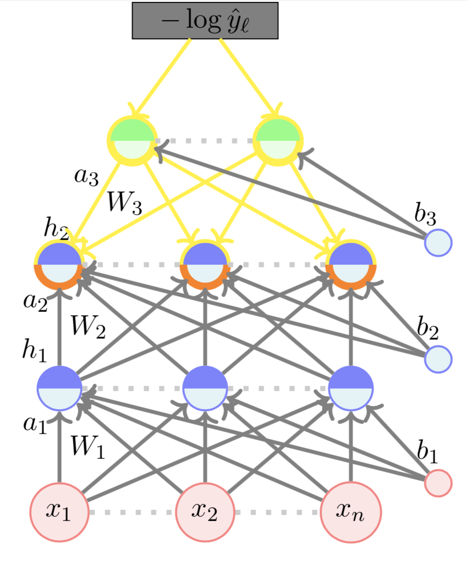
\( \nabla_{a_2} \mathscr{L}(\theta)\) :
W_1 = \begin{bmatrix} 0.1 & 0.3 & 0.8\\ -0.3 & -0.2 & 0.5 \\ -0.3 & 0.1 & 0.4 \\ \end{bmatrix}
W_3 = \begin{bmatrix} 0.3 & -0.5\\ 0.1 & 0.2\\ -0.1 & -0.4\\ \end{bmatrix}
= \begin{bmatrix} \frac{\partial \mathscr{L}{\theta}}{\partial a_{21}} \\ \\ \frac{\partial \mathscr{L}{\theta}}{\partial a_{22 }}\\ \\ \frac{\partial \mathscr{L}{\theta}}{\partial a_{23 }}\\ \end{bmatrix}
= \begin{bmatrix} \textcolor{red}{\frac{\partial \mathscr{L}({\theta})}{\partial h_{21}}} g'(a_{21})\\ \\ \textcolor{red}{\frac{\partial \mathscr{L}({\theta})}{\partial h_{22}}} g'(a_{22})\\ \\ \textcolor{red}{\frac{\partial \mathscr{L}({\theta})}{\partial h_{23}}} g'(a_{23})\\ \end{bmatrix}
= \begin{bmatrix} 0.23 * 0.84\\ \\ - 0.03 * 0.96\\ \\ 0.09 * 0.28 \end{bmatrix}

\( \nabla_{h_2} \mathscr{L}(\theta)\) :

= \begin{bmatrix} \frac{\partial \mathscr{L}{\theta}}{\partial h_{21}} \\ \\ \frac{\partial \mathscr{L}{\theta}}{\partial h_{22 }}\\ \\ \frac{\partial \mathscr{L}{\theta}}{\partial h_{23 }}\\ \end{bmatrix}
= \begin{bmatrix} 0.23\\ \\ - 0.03\\ \\ 0.09 \end{bmatrix}
= \begin{bmatrix} 0.19\\ \\ - 0.03\\ \\ 0.02 \end{bmatrix}

Learning Algorithm


Backward Propogation

W_2 = \begin{bmatrix} 0.4 & 0.5 & -0.3 \\ -0.1 & -0.4 & -0.5\\ 0.8 & 0.2 & 0.9\\ \end{bmatrix}
b = [\ \ 0\ \ \ 0\ \ 0\ \ ]
y = [\ \ 1 \ \ \ 0\ \ ]
x = [\ \ 2\ \ \ 5 \ \ \ 3 \ \ ]

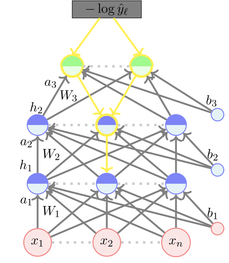
\( \nabla_{W_2} \mathscr{L}(\theta)\) :
W_1 = \begin{bmatrix} 0.1 & 0.3 & 0.8\\ -0.3 & -0.2 & 0.5 \\ -0.3 & 0.1 & 0.4 \\ \end{bmatrix}
W_3 = \begin{bmatrix} 0.3 & -0.5\\ 0.1 & 0.2\\ -0.1 & -0.4\\ \end{bmatrix}
= \begin{bmatrix} \textcolor{red}{\frac{\partial \mathscr{L}{\theta}}{\partial a_{21}}}h_{11} & \textcolor{red}{\frac{\partial \mathscr{L}{\theta}}{\partial a_{21}}}h_{12} & \textcolor{red}{\frac{\partial \mathscr{L}{\theta}}{\partial a_{21}}}h_{13}\\ \\ \textcolor{red}{\frac{\partial \mathscr{L}{\theta}}{\partial a_{22}}}h_{11} & \textcolor{red}{\frac{\partial \mathscr{L}{\theta}}{\partial a_{22}}}h_{12} & \textcolor{red}{\frac{\partial \mathscr{L}{\theta}}{\partial a_{22}}}h_{13}\\ \\ \textcolor{red}{\frac{\partial \mathscr{L}{\theta}}{\partial a_{23}}}h_{11} & \textcolor{red}{\frac{\partial \mathscr{L}{\theta}}{\partial a_{23}}}h_{12} & \textcolor{red}{\frac{\partial \mathscr{L}{\theta}}{\partial a_{23}}}h_{13}\\\\ \end{bmatrix}

\( \nabla_{a_2} \mathscr{L}(\theta)\)

= \begin{bmatrix} -0.19 & 0.03 & -0.02\\ \\ - 0.02 & 0.01 & -0.01\\ \\ 0.2 & -0.03 & 0.02 \\ \end{bmatrix}
= \begin{bmatrix} 0.19\\ \\ - 0.03\\ \\ 0.02 \end{bmatrix}
= \begin{bmatrix} -0.97\\ \\ -0.1\\ \\ 0.99 \end{bmatrix}
h_{1}

Learning Algorithm


Backward Propogation

W_2 = \begin{bmatrix} 0.4 & 0.5 & -0.3 \\ -0.1 & -0.4 & -0.5\\ 0.8 & 0.2 & 0.9\\ \end{bmatrix}
b = [\ \ 0\ \ \ 0\ \ 0\ \ ]
y = [\ \ 1 \ \ \ 0\ \ ]
x = [\ \ 2\ \ \ 5 \ \ \ 3 \ \ ]

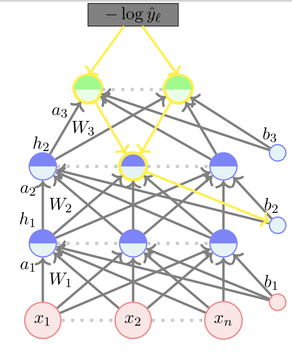
\( \nabla_{b_2} \mathscr{L}(\theta)\) :
W_1 = \begin{bmatrix} 0.1 & 0.3 & 0.8\\ -0.3 & -0.2 & 0.5 \\ -0.3 & 0.1 & 0.4 \\ \end{bmatrix}
W_3 = \begin{bmatrix} 0.3 & -0.5\\ 0.1 & 0.2\\ -0.1 & -0.4\\ \end{bmatrix}
= \textcolor{red}{\nabla_{a_2} \mathscr{L}(\theta)}

\( \nabla_{a_2} \mathscr{L}(\theta)\)

= \begin{bmatrix} 0.19\\ \\ - 0.03\\ \\ 0.02 \end{bmatrix}

Evaluation


How do you check the performance of a deep neural network?

(c) One Fourth Labs

Test  Data

Accuracy=\frac{\text{Number of correct predictions}}{\text{Total number of predictions}}
= \frac{2}{4} = 50\%

Indian Liver Patient Records \(^{*}\)

 -   whether person needs to be diagnosed or not ?

Age
65
62
20
84
Albumin
3.3
3.2
4
3.2
T_Bilirubin
0.7
10.9
1.1
0.7
y
0
0
1
1

.

.

.

Predicted
0
1
1
0

Take-aways

What are the new things that we learned in this module ?

(c) One Fourth Labs


\( x_i \in \mathbb{R} \)

Accuracy=\frac{\text{Number of correct predictions}}{\text{Total number of predictions}}

Loss

Model

Data

Task

Evaluation

Learning

Real inputs

Tasks with Real Inputs and Real Outputs

Back-propagation

Squared Error Loss :

L(\Theta) = \frac{1}{N} \displaystyle\sum_{i=1}^N \displaystyle\sum_{i=1}^d (\hat{y}_{ij} - y_{ij})^2

Cross Entropy Loss:

L(\Theta) = -\frac{1}{N} \displaystyle\sum_{i=1}^N \displaystyle\sum_{i=1}^d y_{ij}\log{(\hat{y}_{ij})}
\hat{y} = \frac{1}{1+e^{-(w_{21}*(\frac{1}{1+e^{- (w_{11}*x_1 + w_{12}*x_2 + b_1)}}) + w_{22}*(\frac{1}{1+e^{- (w_{13}*x_1 + w_{14}*x_2 + b_1)}}) + b_2)}}

Copy of Working Example

By preksha nema

Copy of Working Example

  • 554