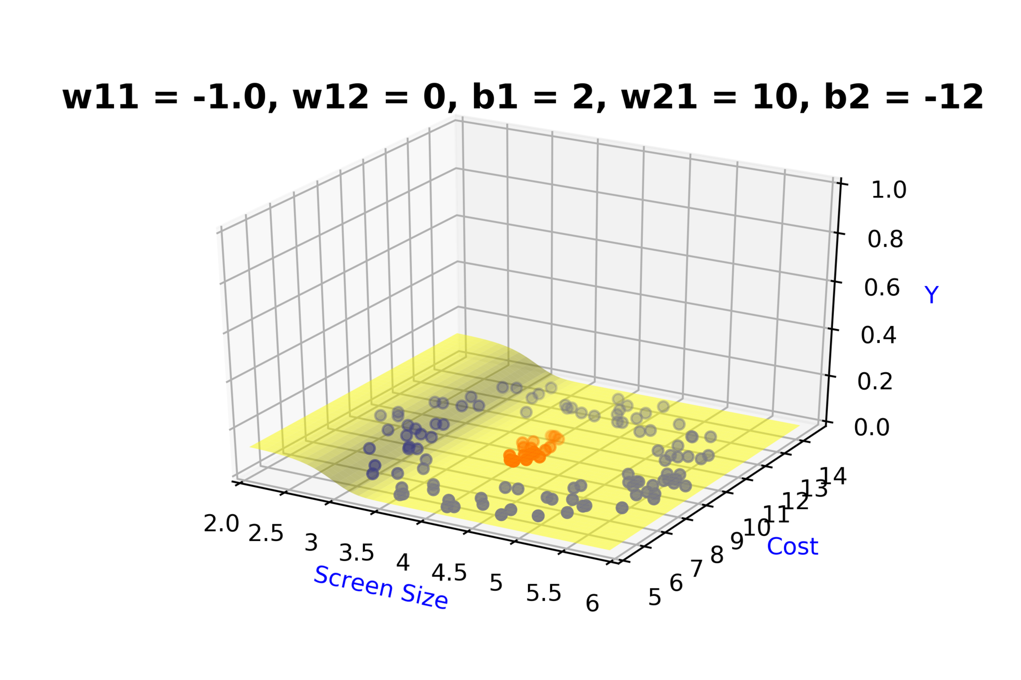
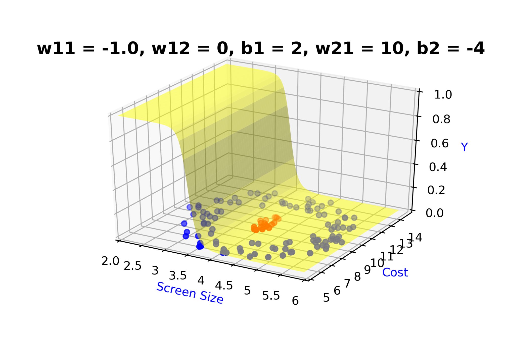
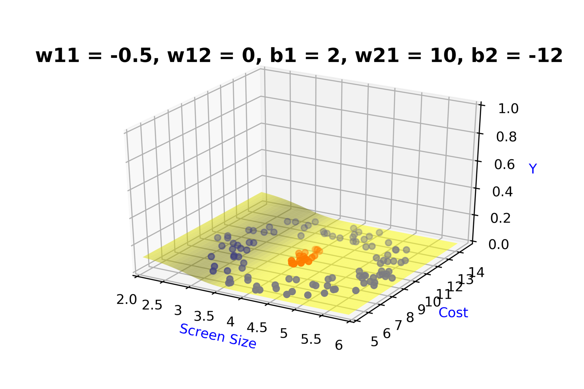
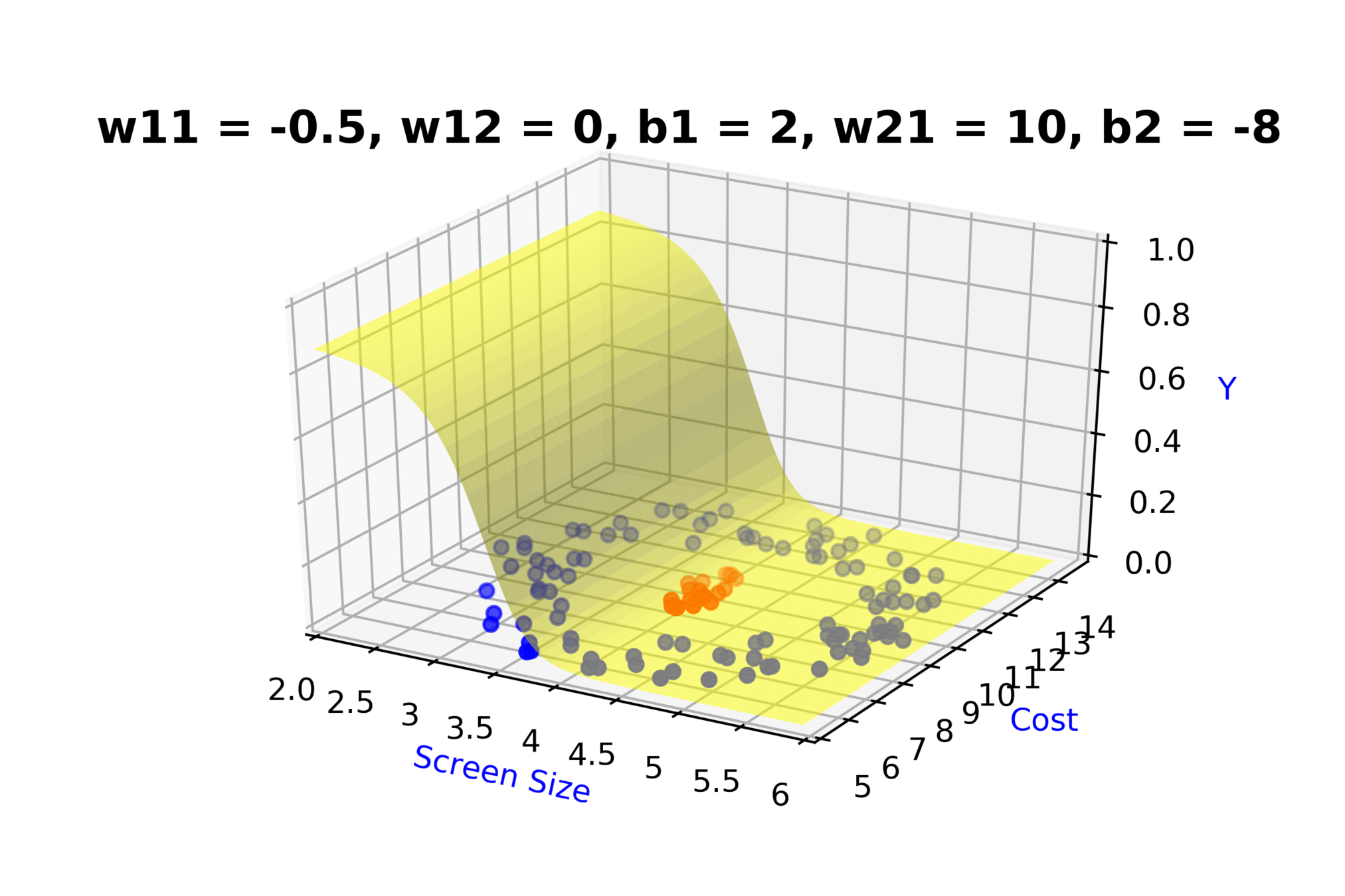
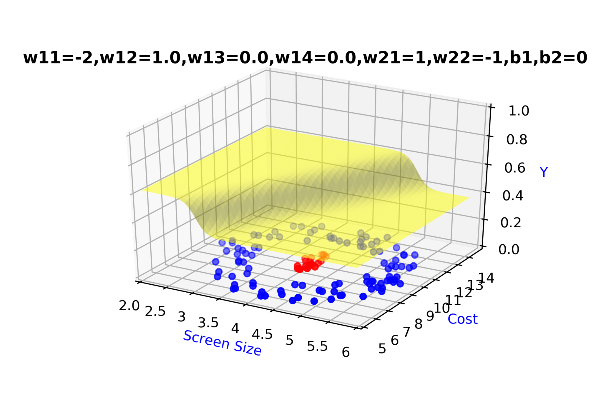
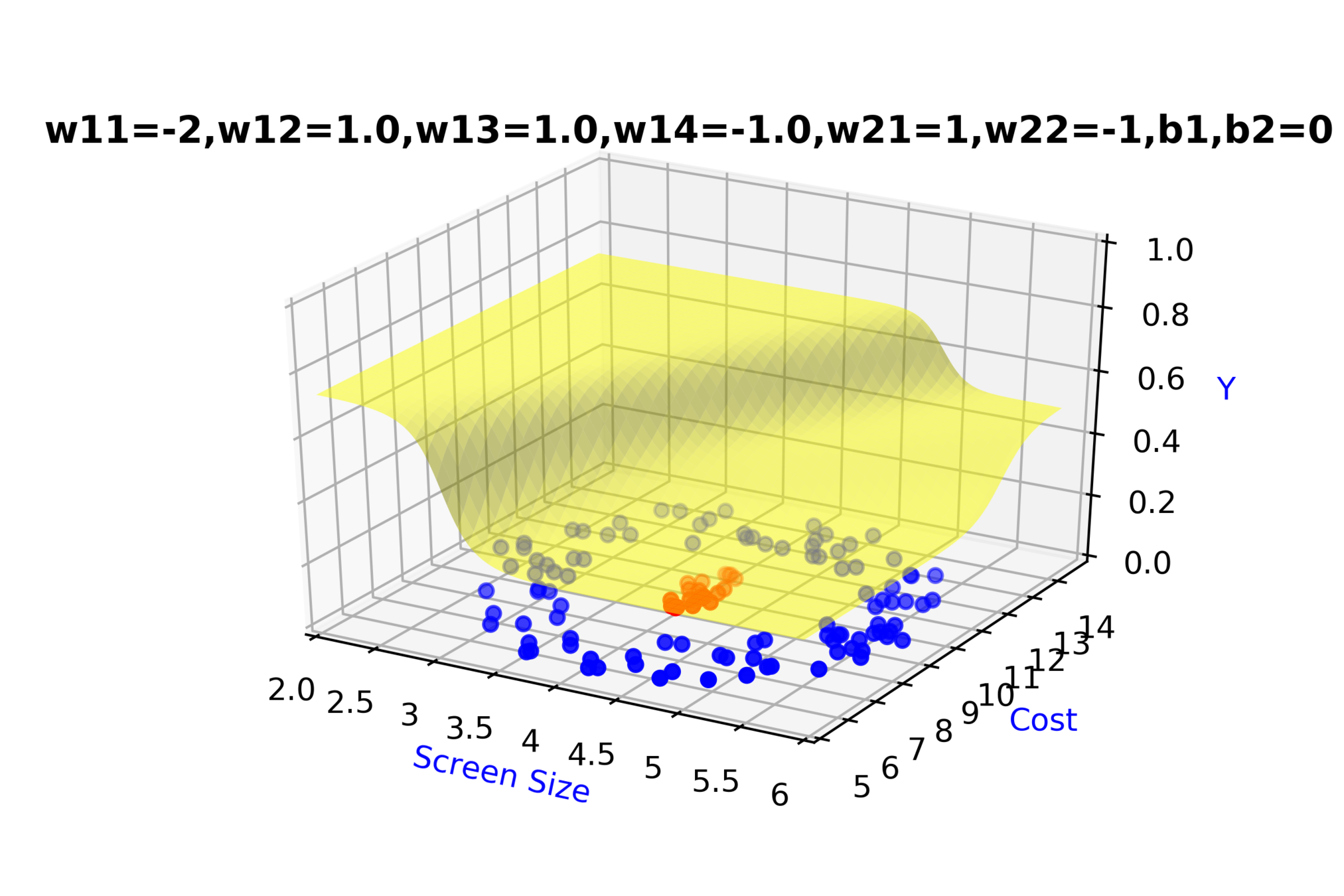
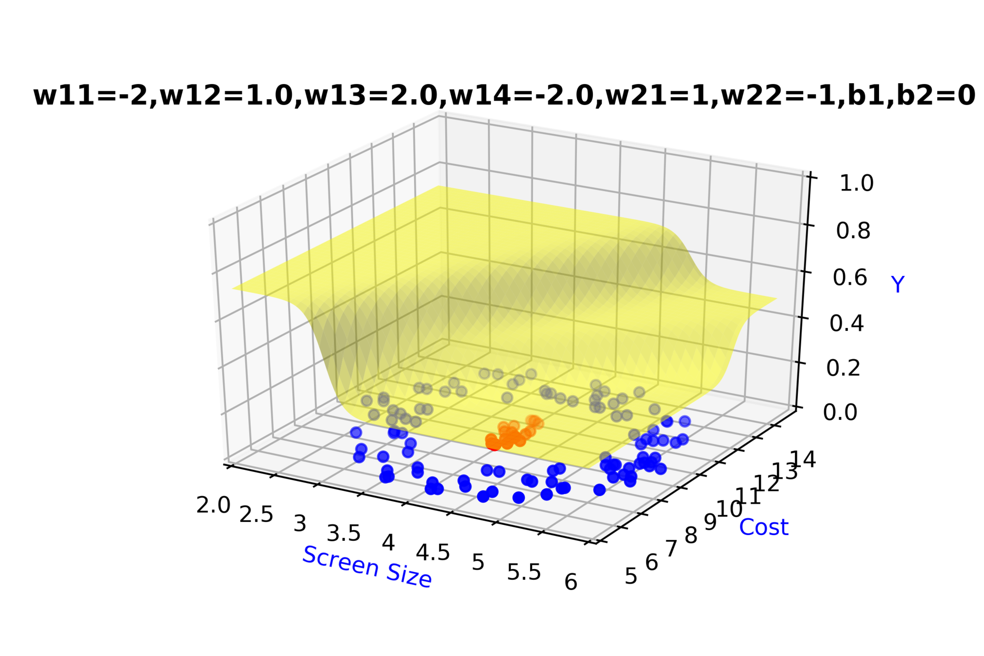
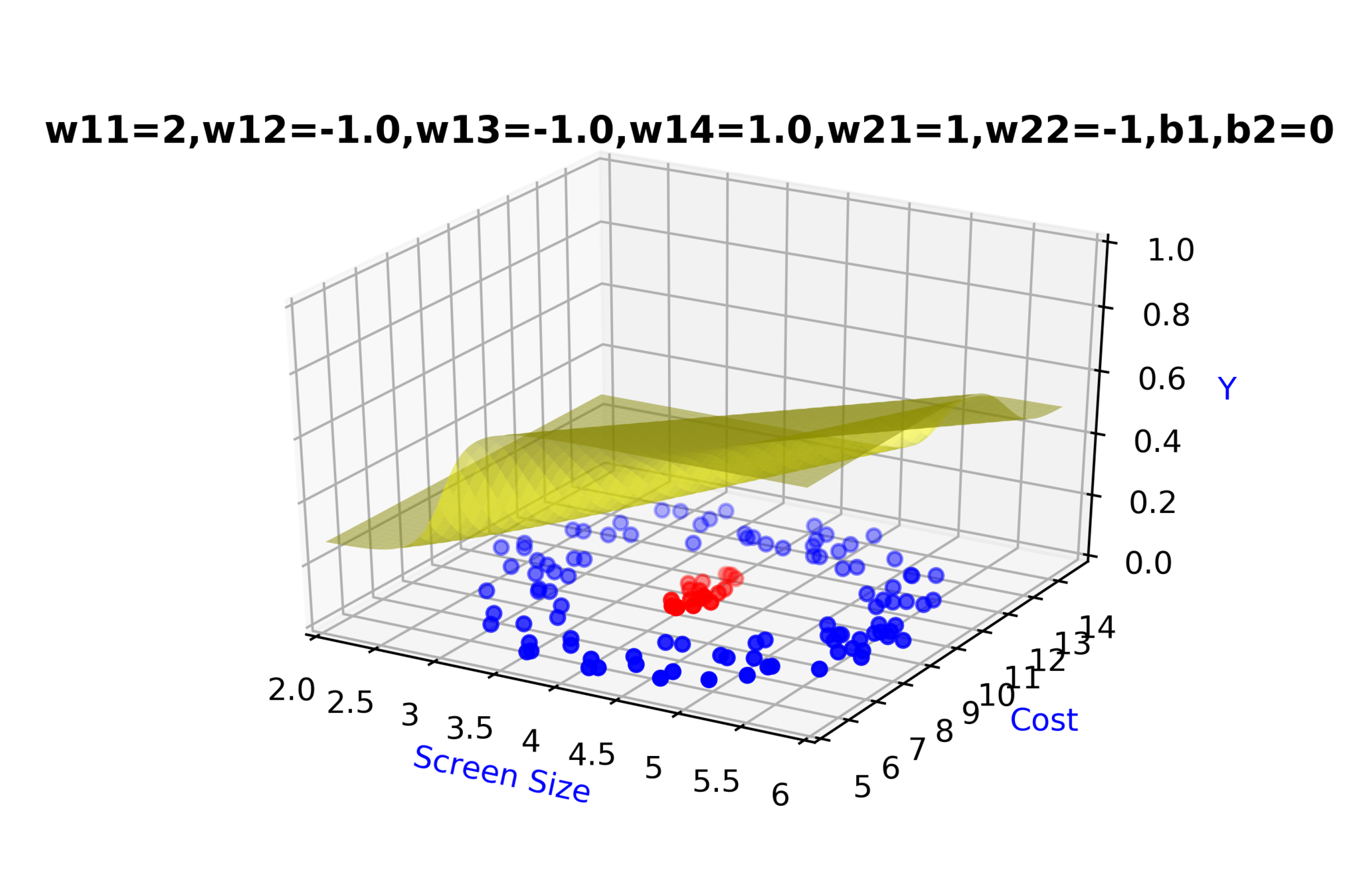
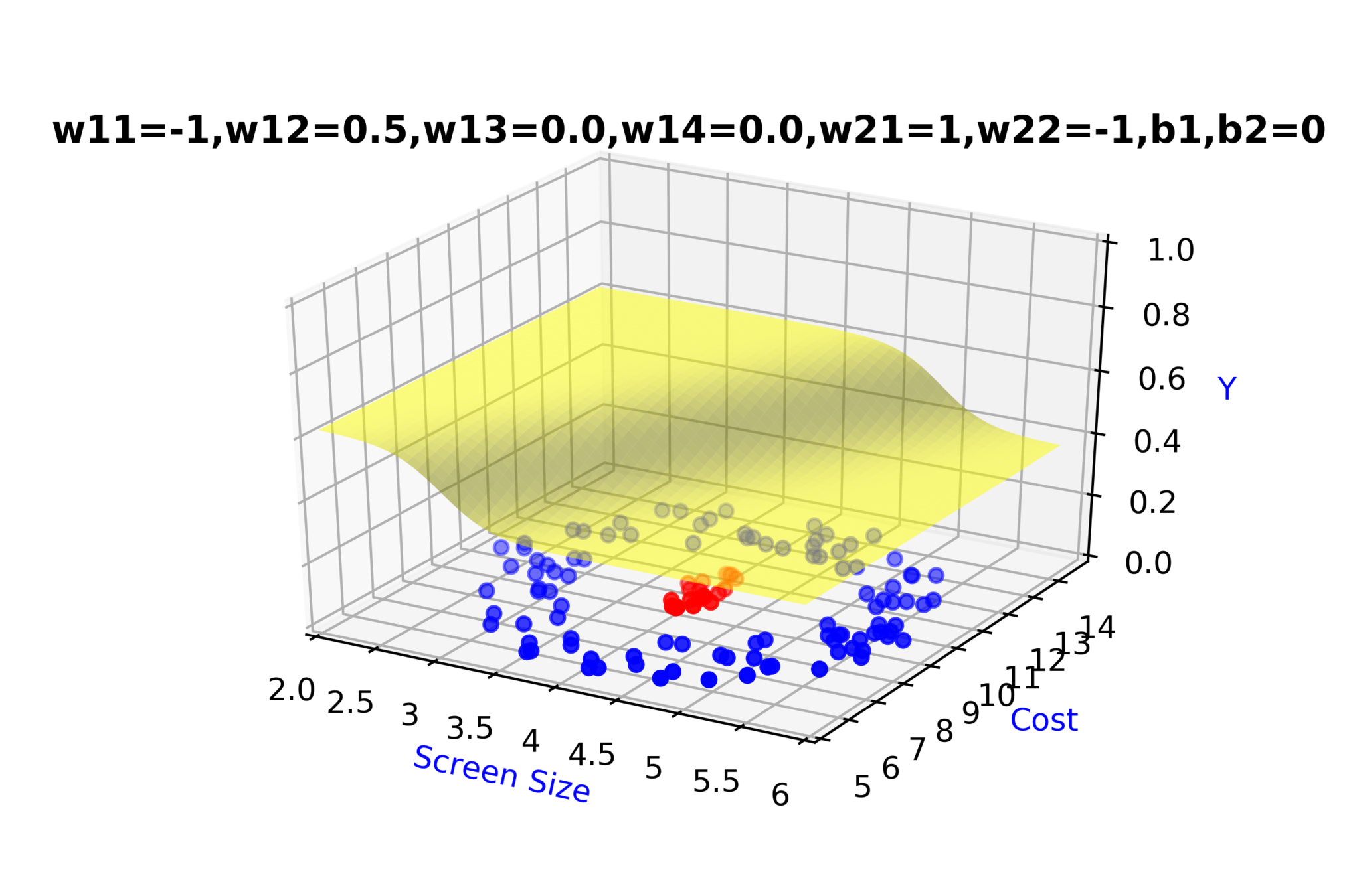
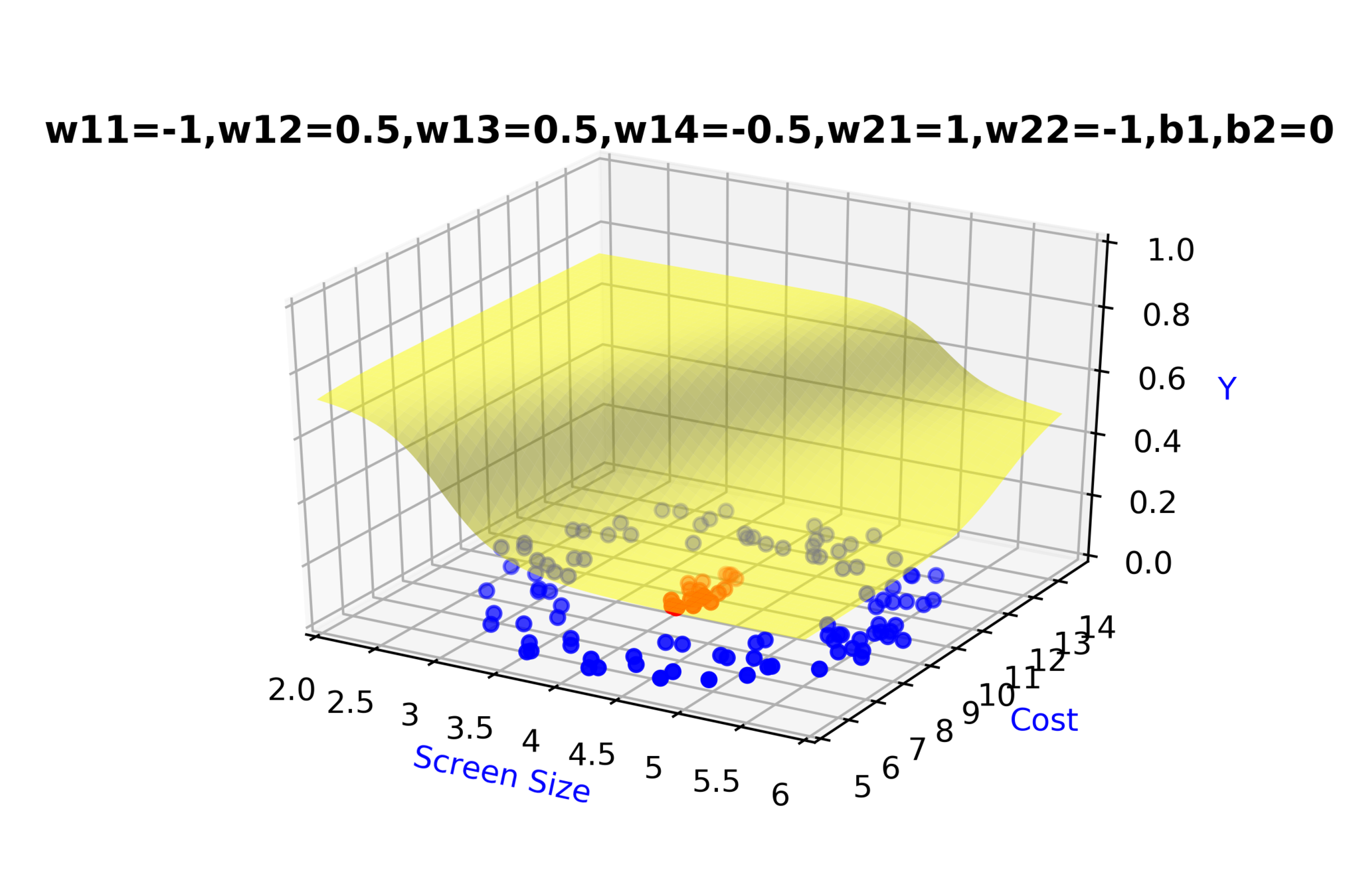
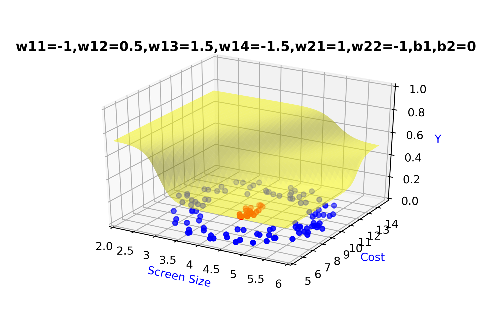
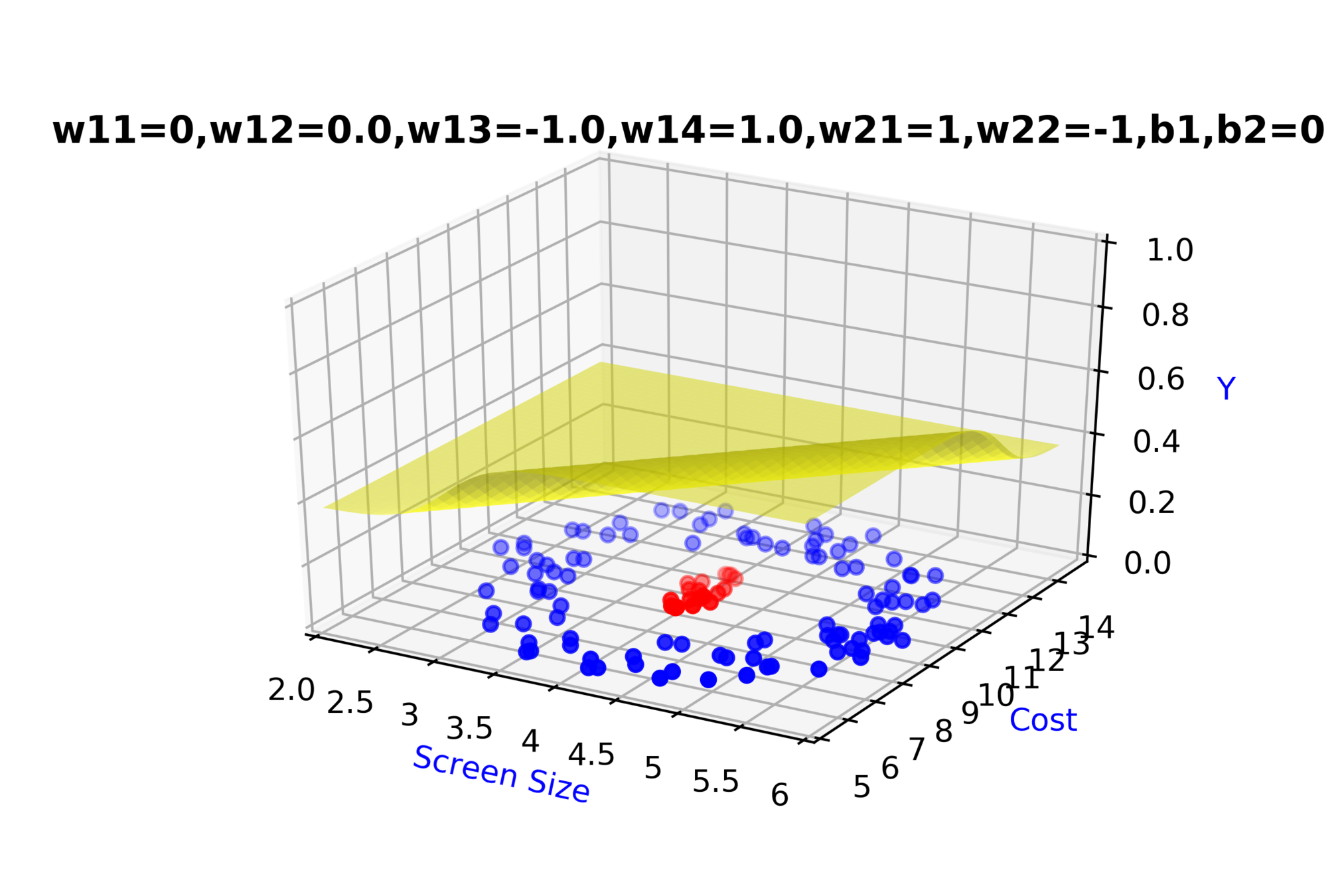
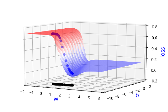
1.9 Multilayered Network of Neurons

Your first Deep Neural Network

Recap: Complex Functions

What we saw in the previous chapter?

(c) One Fourth Labs

Repeat slide 5.1 from the previous lecture 

The Road Ahead

What's going to change now ?

(c) One Fourth Labs

Accuracy=\frac{\text{Number of correct predictions}}{\text{Total number of predictions}}

Loss

Model

Data

Task

Evaluation

Learning

Real inputs

Non-linear

Task specific loss functions

Real outputs

Back-propagation

Data and Task

What kind of data and tasks have DNNs been used for ?

(c) One Fourth Labs

28x28 Images

255
255 183
255 183 95
255 183 95 8 93 196 253
255 183 95 8 93 196 253
254 154 37 7 28 172 254
255 183 95 8 93 196 253
254 154 37 7 28 172 254
252 221 ... ... ... ... ...
... ... ... ... ... ... ...
... ... ... ... ... ... ...
... ... ... ... ... 198 253
252 250 187 178 195 253 253

How can we represent MNIST images as a vector ?

  • Using pixel values of each cell
  • Matrix having pixel values will be of size 28x28             ( As MNIST images are of size 28x28)
  • Each pixel value can range from 0 to 255.  Standardise pixel values by dividing with 255
  • Now, Flatten the matrix to convert into a vector of size 784 (28x28) 
255 183 95 8 93 196 253
254 154 37 7 28 172 254
252 221 ... ... ... ... ...
... ... ... ... ... ... ...
... ... ... ... ... ... ...
... ... ... ... ... 198 253
252 250 187 178 195 253 253
1 183 95 8 93 196 253
254 154 37 7 28 172 254
252 221 ... ... ... ... ...
... ... ... ... ... ... ...
... ... ... ... ... ... ...
... ... ... ... ... 198 253
252 250 187 178 195 253 253
1 0.72 95 8 93 196 253
254 154 37 7 28 172 254
252 221 ... ... ... ... ...
... ... ... ... ... ... ...
... ... ... ... ... ... ...
... ... ... ... ... 198 253
252 250 187 178 195 253 253
1 0.72 0.37 8 93 196 253
254 154 37 7 28 172 254
252 221 ... ... ... ... ...
... ... ... ... ... ... ...
... ... ... ... ... ... ...
... ... ... ... ... 198 253
252 250 187 178 195 253 253
1 0.72 0.37 0.03 0.36 0.77 0.99
254 154 37 7 28 172 254
252 221 ... ... ... ... ...
... ... ... ... ... ... ...
... ... ... ... ... ... ...
... ... ... ... ... 198 253
252 250 187 178 195 253 253
1 0.72 0.37 0.03 0.36 0.77 0.99
1 0.60 0.14 0.03 0.11 0.67 1
252 221 ... ... ... ... ...
... ... ... ... ... ... ...
... ... ... ... ... ... ...
... ... ... ... ... 198 253
252 250 187 178 195 253 253
1 0.72 0.37 0.03 0.36 0.77 0.99
1 0.60 0.14 0.03 0.11 0.67 1
0.99 0.87 ... ... ... ... ...
... ... ... ... ... ... ...
... ... ... ... ... ... ...
... ... ... ... ... 0.78 0.99
0.99 0.98 0.73 0.69 0.76 0.99 0.99

Data and Task

What kind of data and tasks have DNNs been used for ?

(c) One Fourth Labs

28x28 Images

How can we represent MNIST images as a vector ?

  • Using pixel values of each cell
  • Matrix having pixel values will be of size 28x28             ( As MNIST images are of size 28x28)
  • Each pixel value can range from 0 to 255.  Standardise pixel values by dividing with 255
  • Now, Flatten the matrix to convert into a vector of size 784 (28x28) 

\( \left[\begin{array}{lcr} 1.00, 0.72, 0.37 \dots, 0.76, 0.99, 0.99 \end{array} \right]\)

\( \left[\begin{array}{lcr} 1.00, 0.85, 0.73 \dots, 0.68, 1.00, 1.00 \end{array} \right]\)

\( \left[\begin{array}{lcr} 1.00, 0.76, 0.64 \dots, 0.86, 0.99, 1.00 \end{array} \right]\)

\( \left[\begin{array}{lcr} 0.99, 0.82, 0.26 \dots, 0.53, 0.87, 1.00 \end{array} \right]\)

\( \left[\begin{array}{lcr} 0.73, 0.81, 0.87 \dots, 0.76, 0.79, 0.67 \end{array} \right]\)

\( \left[\begin{array}{lcr} 0.84, 0.72, 0.31 \dots, 0.26, 0.51, 0.99 \end{array} \right]\)

\( \left[\begin{array}{lcr} 1.00, 1.00, 0.96 \dots, 0.88, 0.79, 0.99 \end{array} \right]\)

\( \left[\begin{array}{lcr} 0.33, 0.52, 0.47 \dots, 0.76, 0.95, 1.00 \end{array} \right]\)

\( \left[\begin{array}{lcr} 0.85, 0.72, 0.97 \dots, 0.86, 0.94, 0.99 \end{array} \right]\)

\( \left[\begin{array}{lcr} 0.84, 0.92, 0.28 \dots, 0.76, 1.0, 0.99 \end{array} \right]\)

Data and Task

What kind of data and tasks have DNNs been used for ?

(c) One Fourth Labs

28x28 Images

\( \left[\begin{array}{lcr} 1.00, 0.72, 0.37 \dots, 0.76, 0.99, 0.99 \end{array} \right]\)

\( \left[\begin{array}{lcr} 1.00, 0.85, 0.73 \dots, 0.68, 1.00, 1.00 \end{array} \right]\)

\( \left[\begin{array}{lcr} 1.00, 0.76, 0.64 \dots, 0.86, 0.99, 1.00 \end{array} \right]\)

\( \left[\begin{array}{lcr} 0.99, 0.82, 0.26 \dots, 0.53, 0.87, 1.00 \end{array} \right]\)

\( \left[\begin{array}{lcr} 0.73, 0.81, 0.87 \dots, 0.76, 0.79, 0.67 \end{array} \right]\)

\( \left[\begin{array}{lcr} 0.84, 0.72, 0.31 \dots, 0.26, 0.51, 0.99 \end{array} \right]\)

\( \left[\begin{array}{lcr} 1.00, 1.00, 0.96 \dots, 0.88, 0.79, 0.99 \end{array} \right]\)

\( \left[\begin{array}{lcr} 0.33, 0.52, 0.47 \dots, 0.76, 0.95, 1.00 \end{array} \right]\)

\( \left[\begin{array}{lcr} 0.85, 0.72, 0.97 \dots, 0.86, 0.94, 0.99 \end{array} \right]\)

\( \left[\begin{array}{lcr} 0.84, 0.92, 0.28 \dots, 0.76, 1.00, 0.99 \end{array} \right]\)

Class Label

0

1

2

3

4

5

6

7

8

9

Class labels can be represented as one hot vectors

Class Labels - One hot Representation

\( \left[\begin{array}{lcr} 1, 0, 0, 0, 0, 0, 0, 0, 0, 0 \end{array} \right]\)

\( \left[\begin{array}{lcr} 0, 1, 0, 0, 0, 0, 0, 0, 0, 0 \end{array} \right]\)

\( \left[\begin{array}{lcr} 0, 0, 1, 0, 0, 0, 0, 0, 0, 0 \end{array} \right]\)

\( \left[\begin{array}{lcr} 0, 0, 0, 1, 0, 0, 0, 0, 0, 0 \end{array} \right]\)

\( \left[\begin{array}{lcr} 0, 0, 0, 0, 1, 0, 0, 0, 0, 0 \end{array} \right]\)

\( \left[\begin{array}{lcr} 0, 0, 0, 0, 0, 1, 0, 0, 0, 0 \end{array} \right]\)

\( \left[\begin{array}{lcr} 0, 0, 0, 0, 0, 0, 1, 0, 0, 0 \end{array} \right]\)

\( \left[\begin{array}{lcr} 0, 0, 0, 0, 0, 0, 0, 1, 0, 0 \end{array} \right]\)

\( \left[\begin{array}{lcr} 0, 0, 0, 0, 0, 0, 0, 0, 1, 0 \end{array} \right]\)

\( \left[\begin{array}{lcr} 0, 0, 0, 0, 0, 0, 0, 0, 0, 1 \end{array} \right]\)

Data and Task

What kind of data and tasks have DNNs been used for ?

(c) One Fourth Labs

- Now have two more slides on other Kaggle tasks for which DNNs have been tried (preferably, some non-image tasks and at least one regression task. You could also repeat the churn prediction task from before)


- Finally have 1 slide on our task which is multi character classification

- Same layout and animations repeated from the previous slide only data changes

- Show MNIST dataset sample on LHS

- Show by animation how you will flatten each image and convert it to a vector (of course you cannot show that

Data and Task

What kind of data and tasks have DNNs been used for ?

(c) One Fourth Labs

(c) One Fourth Labs

Indian Liver Patient Records \(^{*}\)

 -   whether person needs to be diagnosed or not ?

Age
65
62
20
84
Albumin
3.3
3.2
4
3.2
T_Bilirubin
0.7
10.9
1.1
0.7
D
0
0
1
1

\( \hat{y} = \hat{f}(x_1, x_2, .... ,x_{N}) \)

\( \hat{D} = \hat{f}(Age, Albumin,T\_Bilirubin,.....) \)

.

.

.

.

.

.

.

.

.

.

.

.

.

.

.

.

.

.

.

.

.

.

.

Data and Task

What kind of data and tasks have DNNs been used for ?

(c) One Fourth Labs

(c) One Fourth Labs

* https://www.kaggle.com/c/boston-housing

Boston Housing\(^{*}\)

- Predict Housing Values in Suburbs of Boston

Crime
 
0.00632
0.02731
0.3237
0.6905
Avg No of rooms
6.575
6.421
6.998
7.147
Age
 
65.2
78.9
45.8
54.2
House Value
 
24
21.6
33.4
36.2

\( \hat{y} = \hat{f}(x_1, x_2, .... ,x_{N}) \)

\( \hat{D} = \hat{f}(Crime, Avg \ no \ of \ rooms, Age, .... ) \)

.

.

.

.

.

.

.

.

.

.

.

.

.

.

.

.

.

.

.

.

.

.

.

Model

How to build complex functions using Deep Neural Networks?

(c) One Fourth Labs

\(x_2\)

Cost

3.5

8k

12k
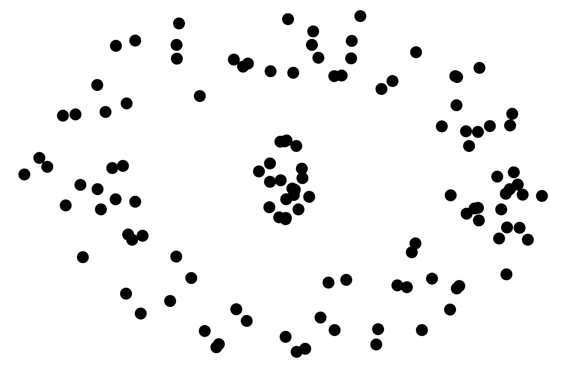
\( \hat{y} = \frac{1}{1+e^{-(w_1* x_1 + w_2*x_2+b)}} \)

\(w_1\)

\(w_2\)

\(x_2\)

\(x_1\)

\( \hat{y} \)

4.5

Screen size

\(x_1\)

\(b\)

\(w_{11}\)

\( \hat{y} = f(x_1,x_2) \)

Model

How to build complex functions using Deep Neural Networks?

(c) One Fourth Labs

\(x_2\)

Cost

3.5

8k

12k
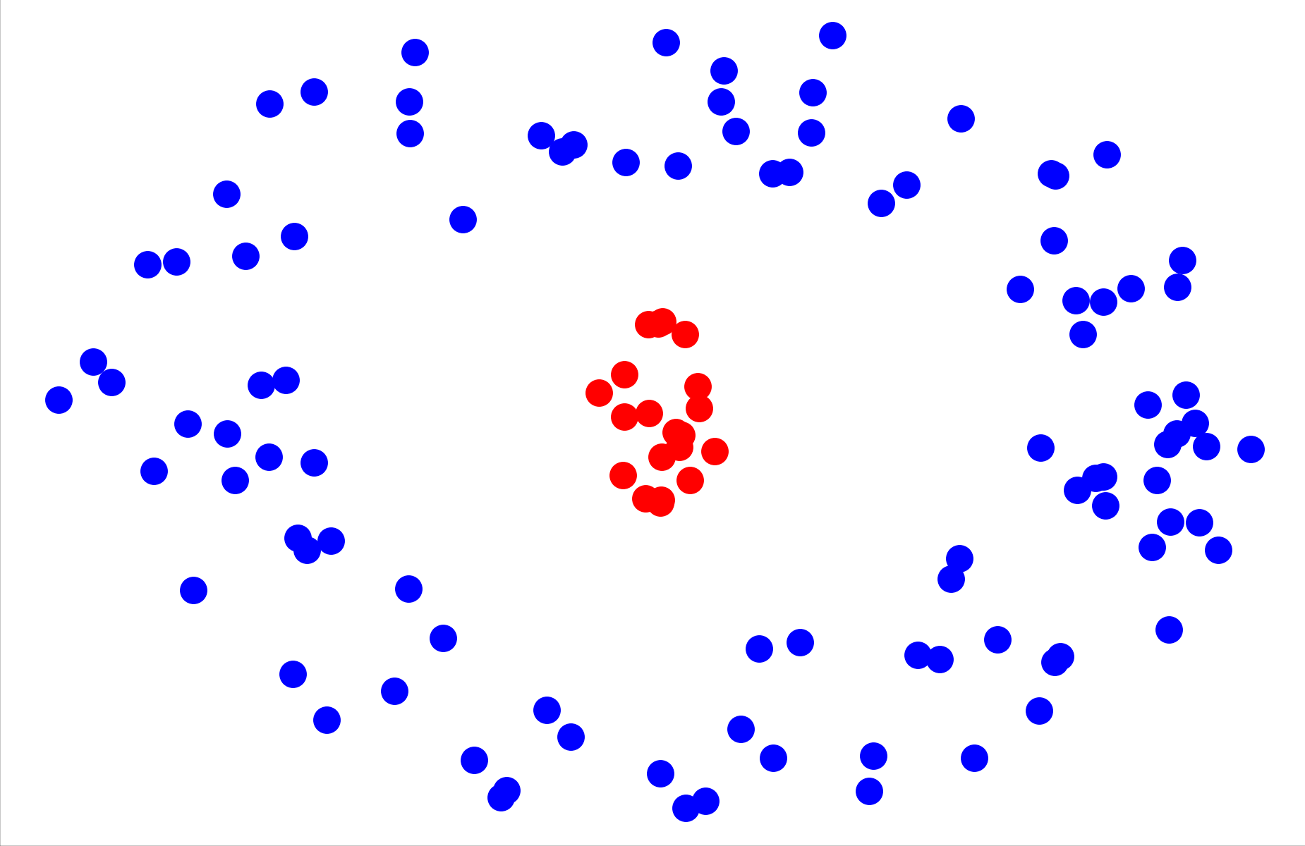
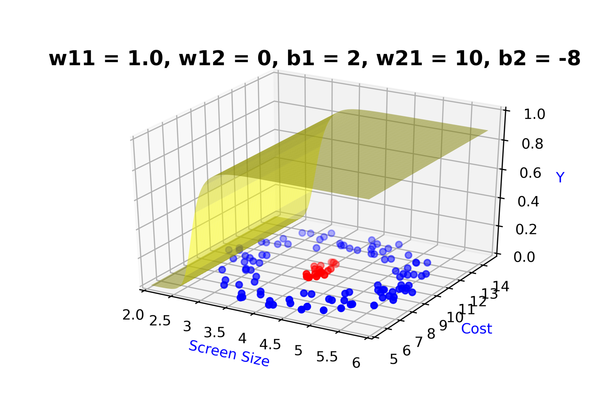
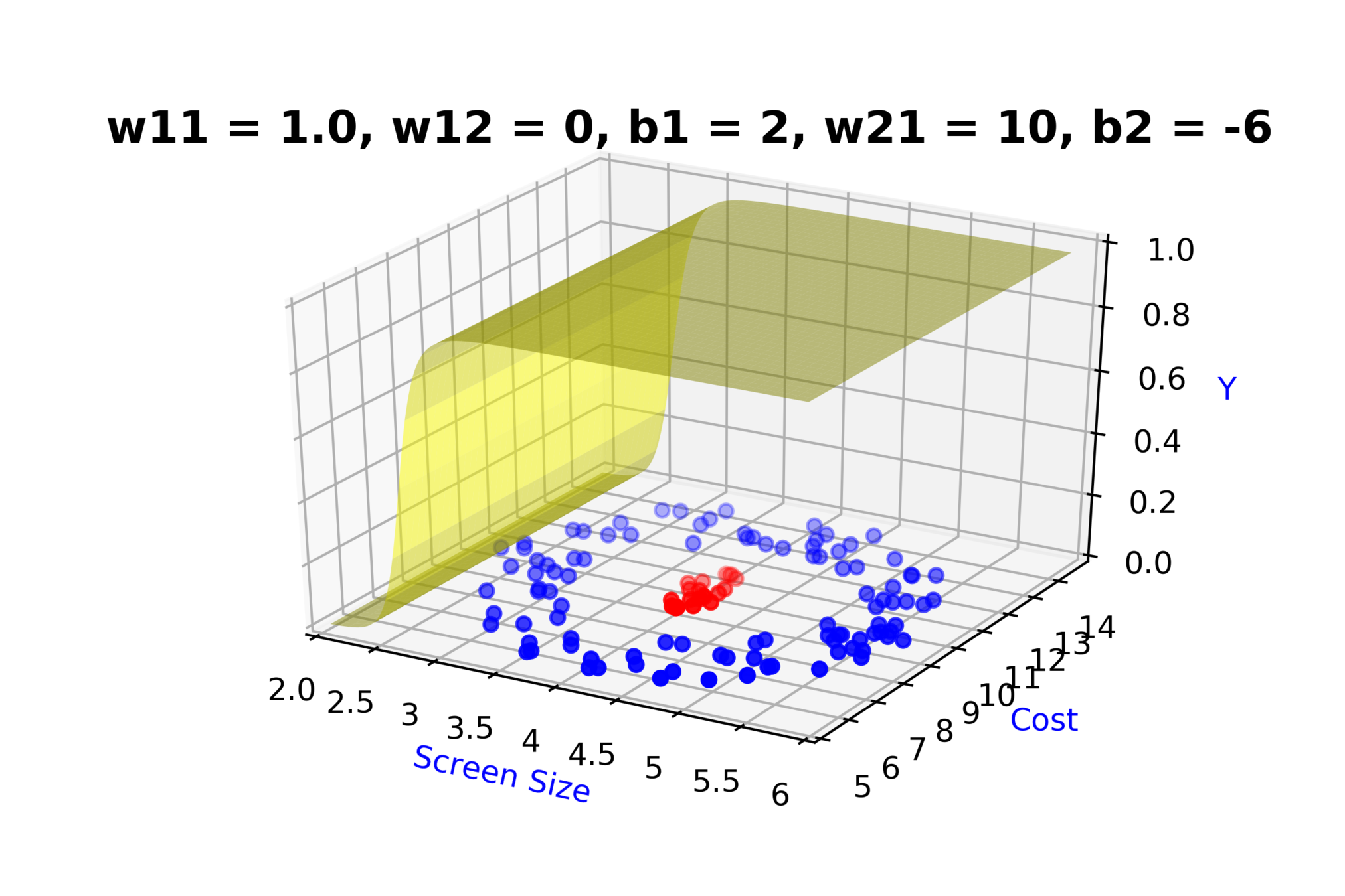
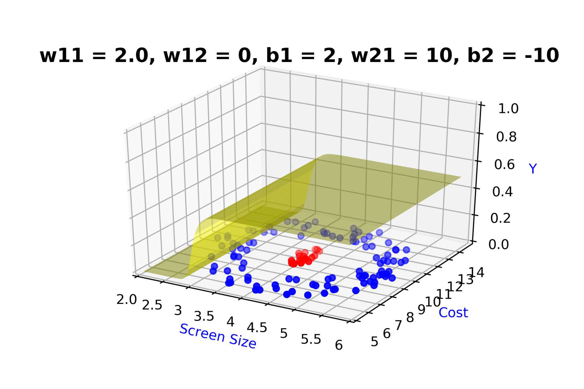
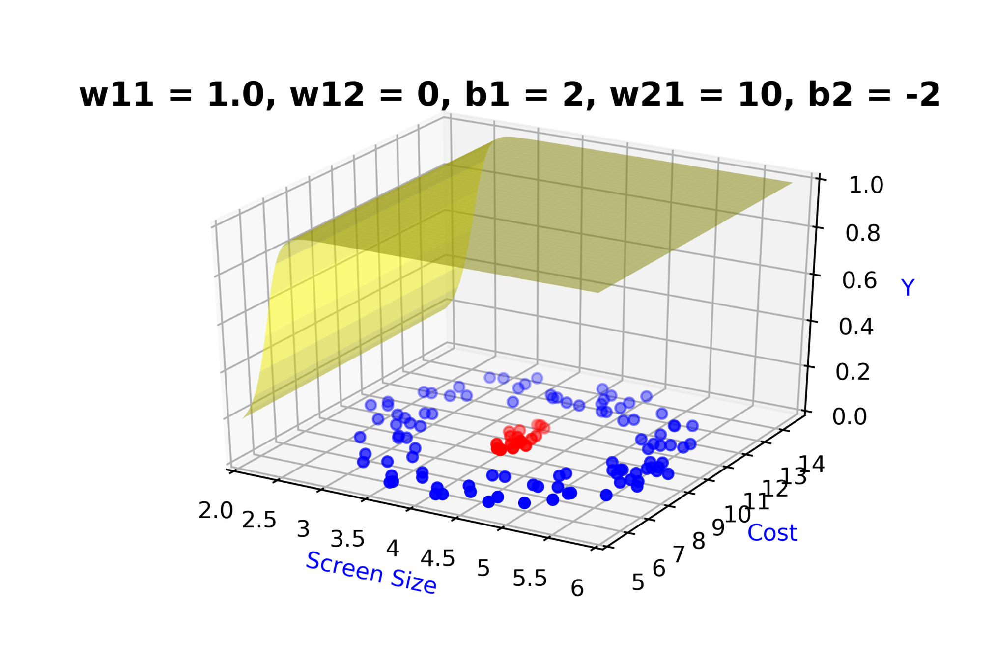
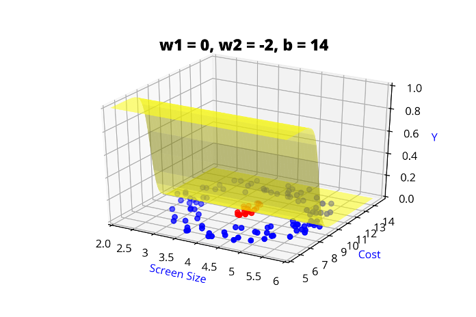
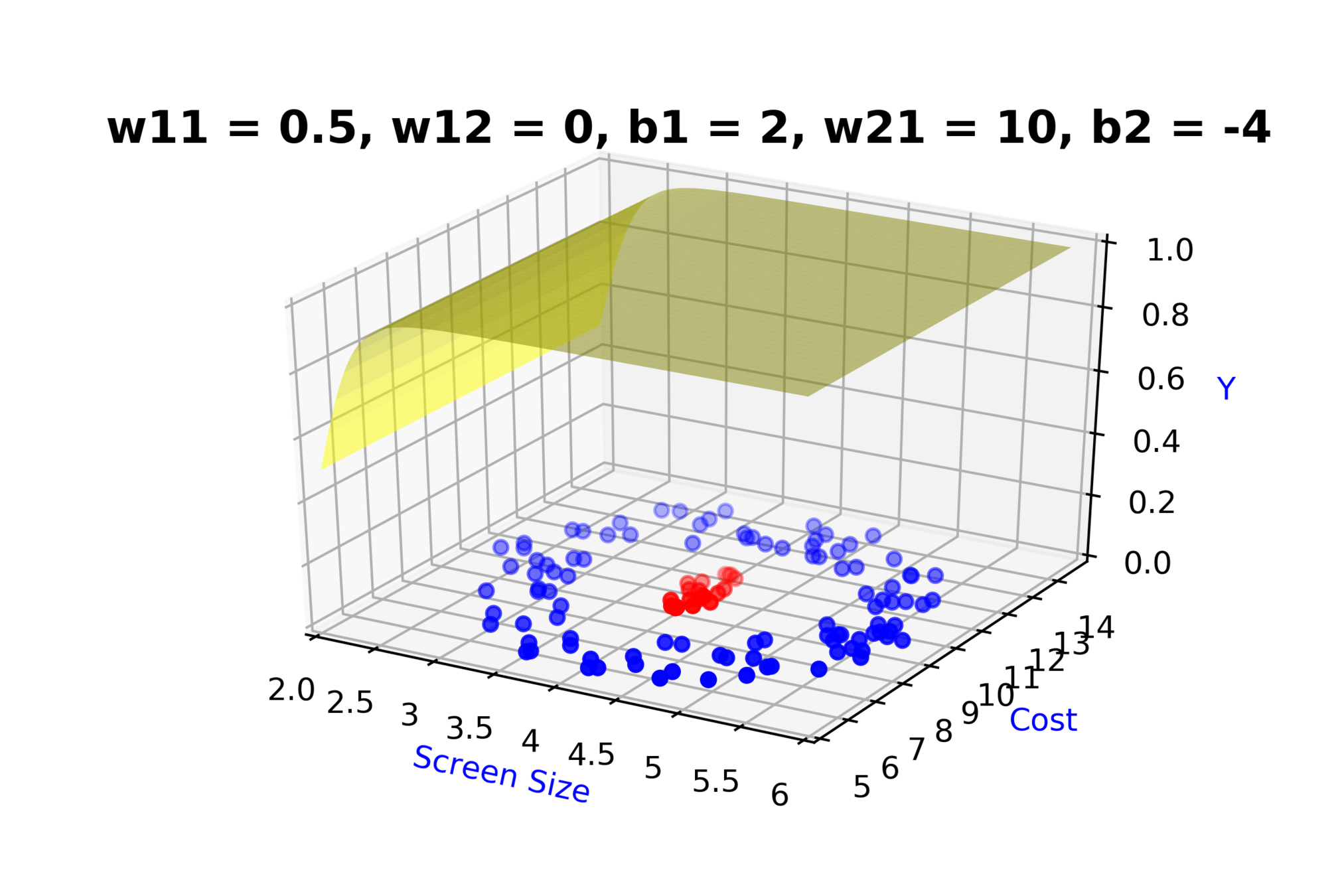
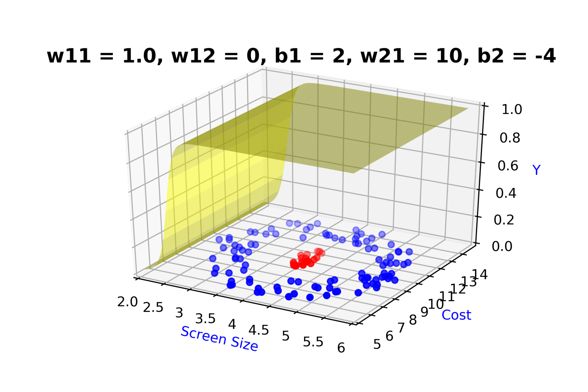
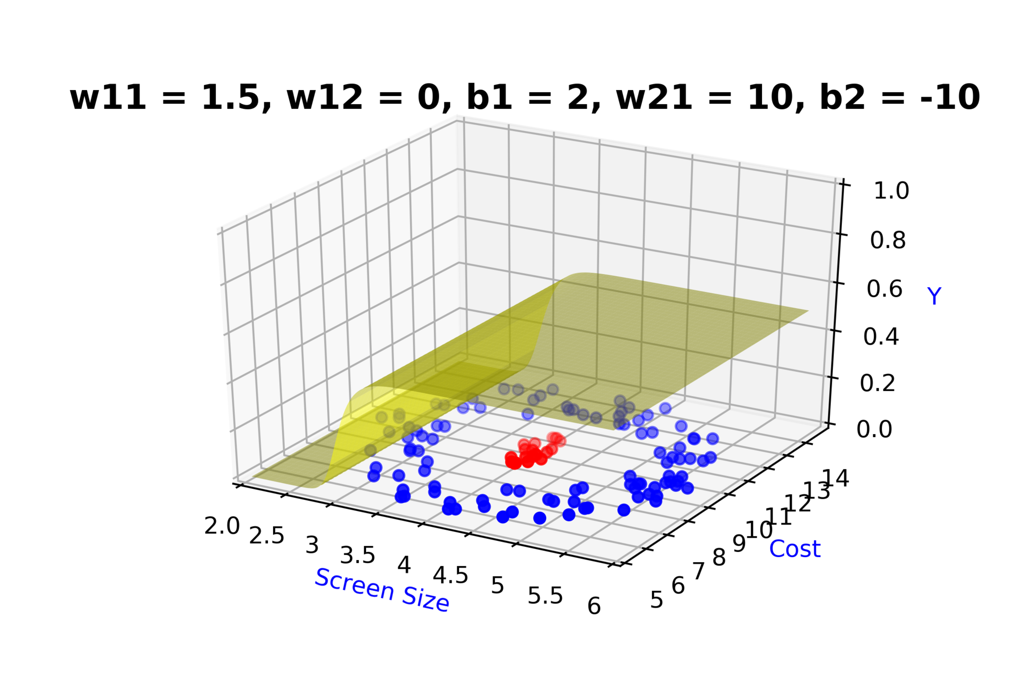
\( h = f(x_1,x_2) \)

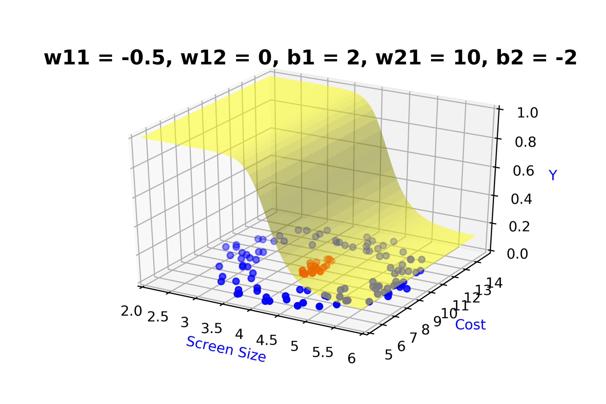
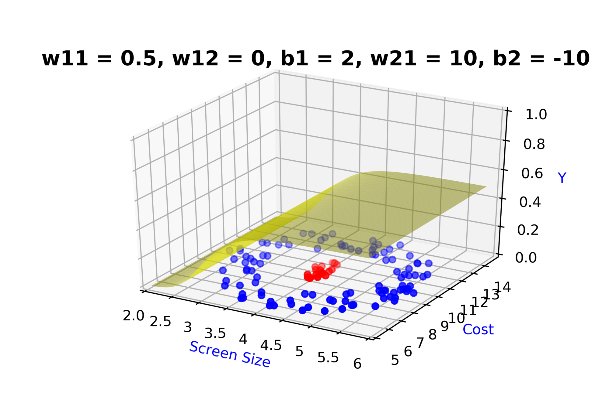
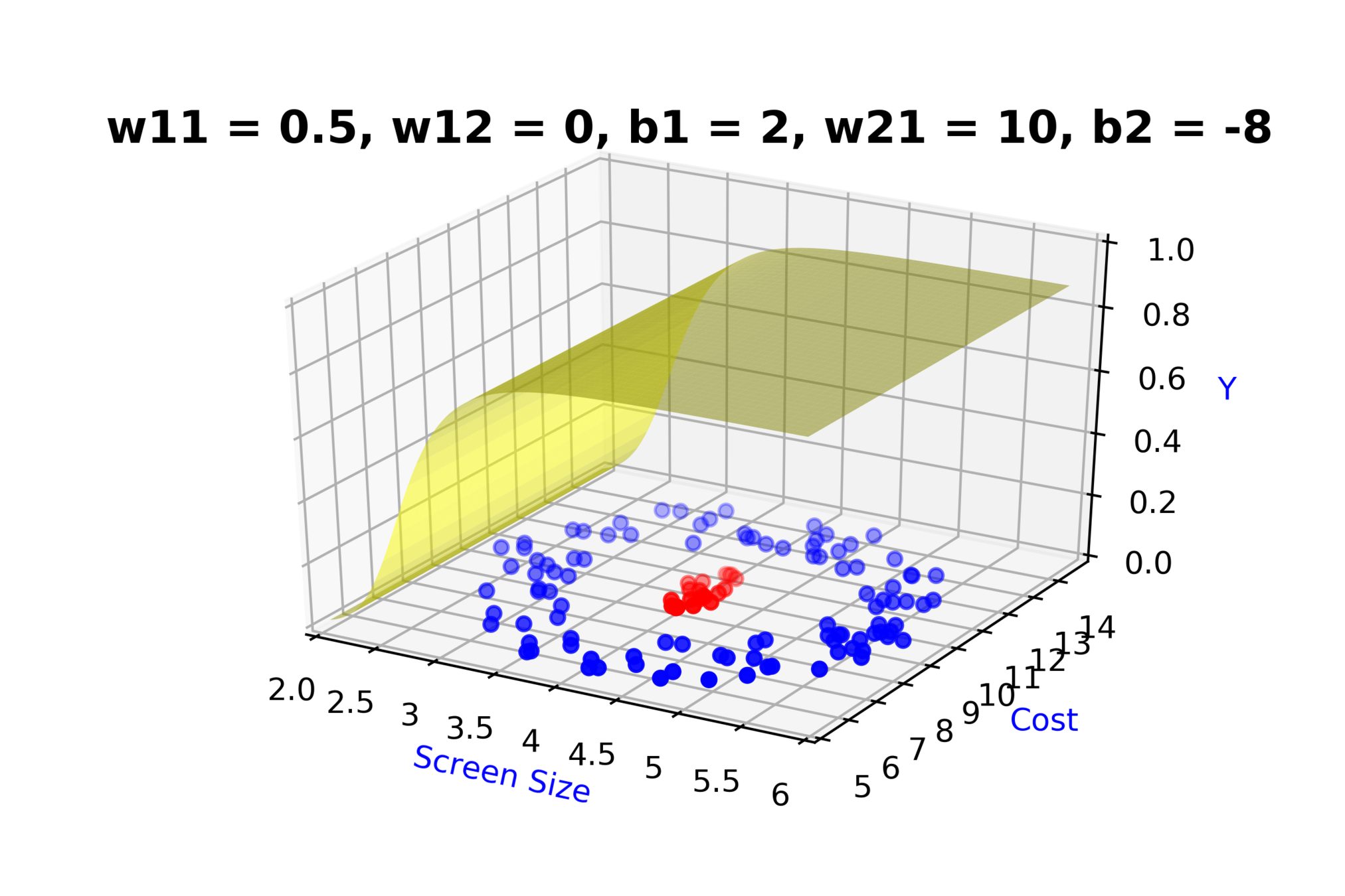
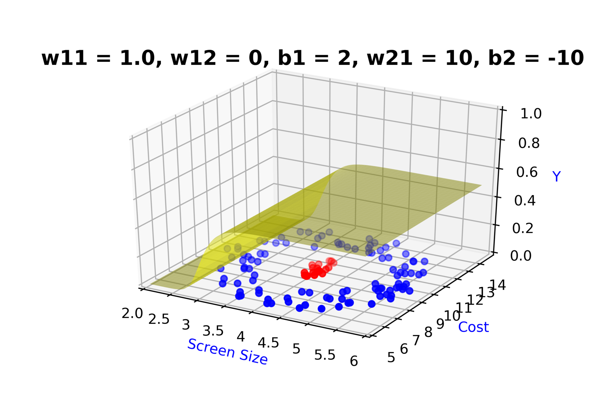
\( h = \frac{1}{1+e^{-(w_{11}* x_1 + w_{12}*x_2+b_1)}} \)

\(w_{11}\)

\(w_{12}\)

\(x_2\)

\(x_1\)

\( \hat{y} \)

4.5

Screen size

\(x_1\)

\(b_1\)

\(b_2\)

\(w_{21}\)

\( \hat{y} = g(h) \)

\( = g(f(x_{1},x_{2})) \)

\(\hat{y} = \frac{1}{1+e^{-(w_{21}*h + b_2)}}\)

= \frac{1}{1+e^{-(w_{21}*(\frac{1}{1+e^{- (w_{11}*x_1 + w_{12}*x_2 + b_1)}}) + b_2)}}

Model

How to build complex functions using Deep Neural Networks?

(c) One Fourth Labs

\(x_2\)

Cost

3.5

8k

12k
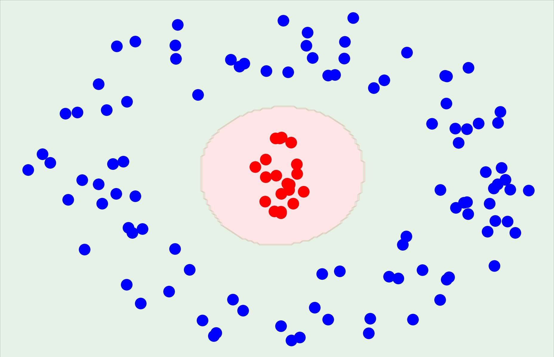
\( h_1 = f_1(x_1,x_2) \)

\( h_1 = \frac{1}{1+e^{-(w_{11}* x_1 + w_{12}*x_2+b_1)}} \)

\(w_{11}\)

\(w_{12}\)

\(x_2\)

\(x_1\)

\( \hat{y} \)
4.5

Screen size

\(x_1\)

\(b_1\)

\(b_2\)

\(w_{21}\)

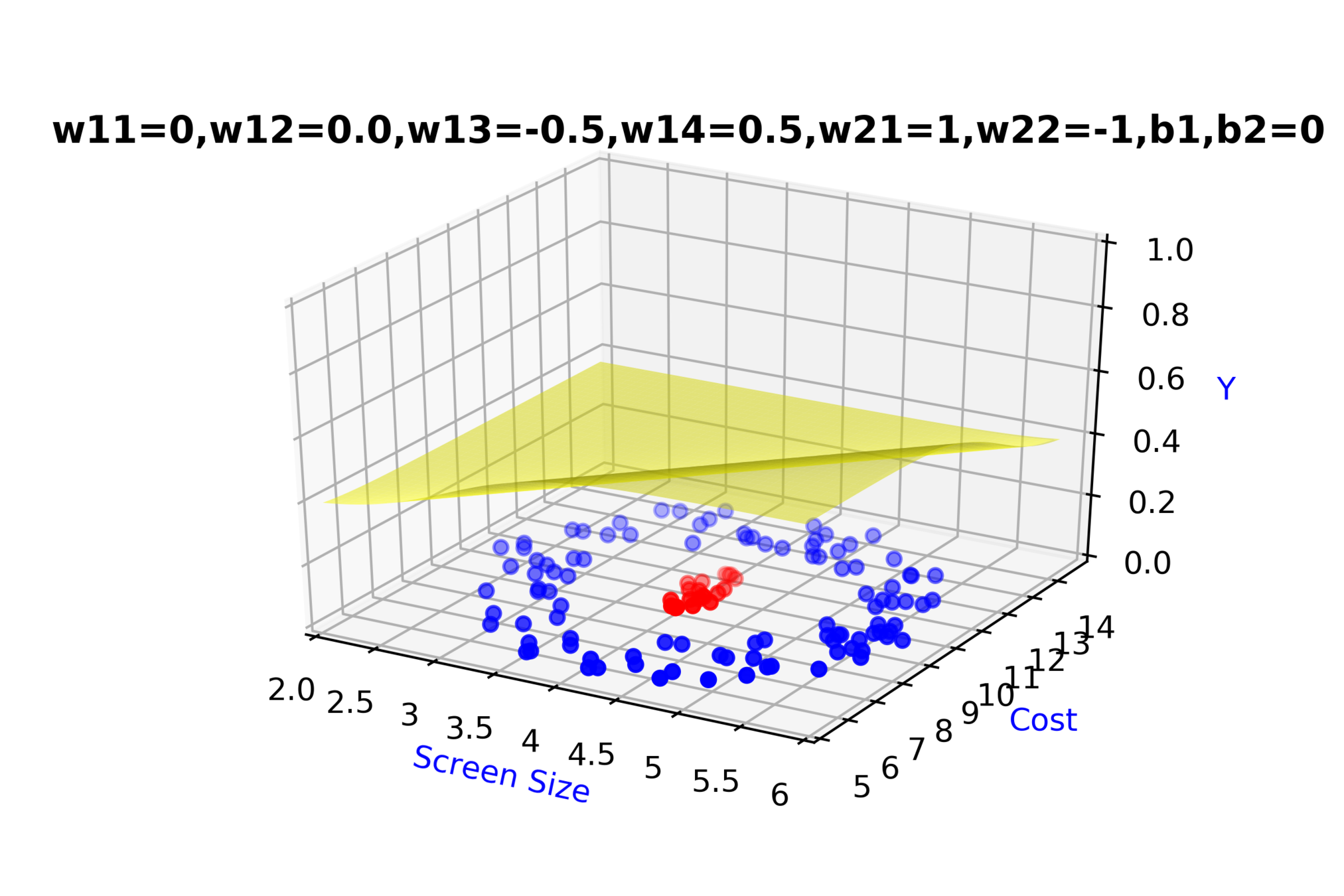
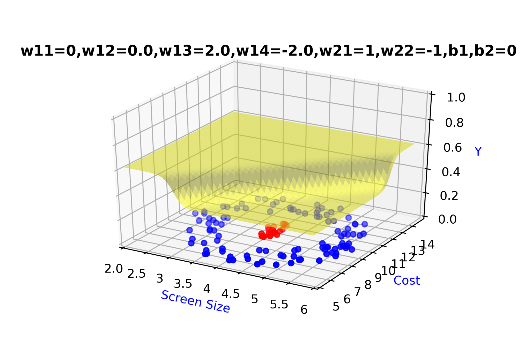
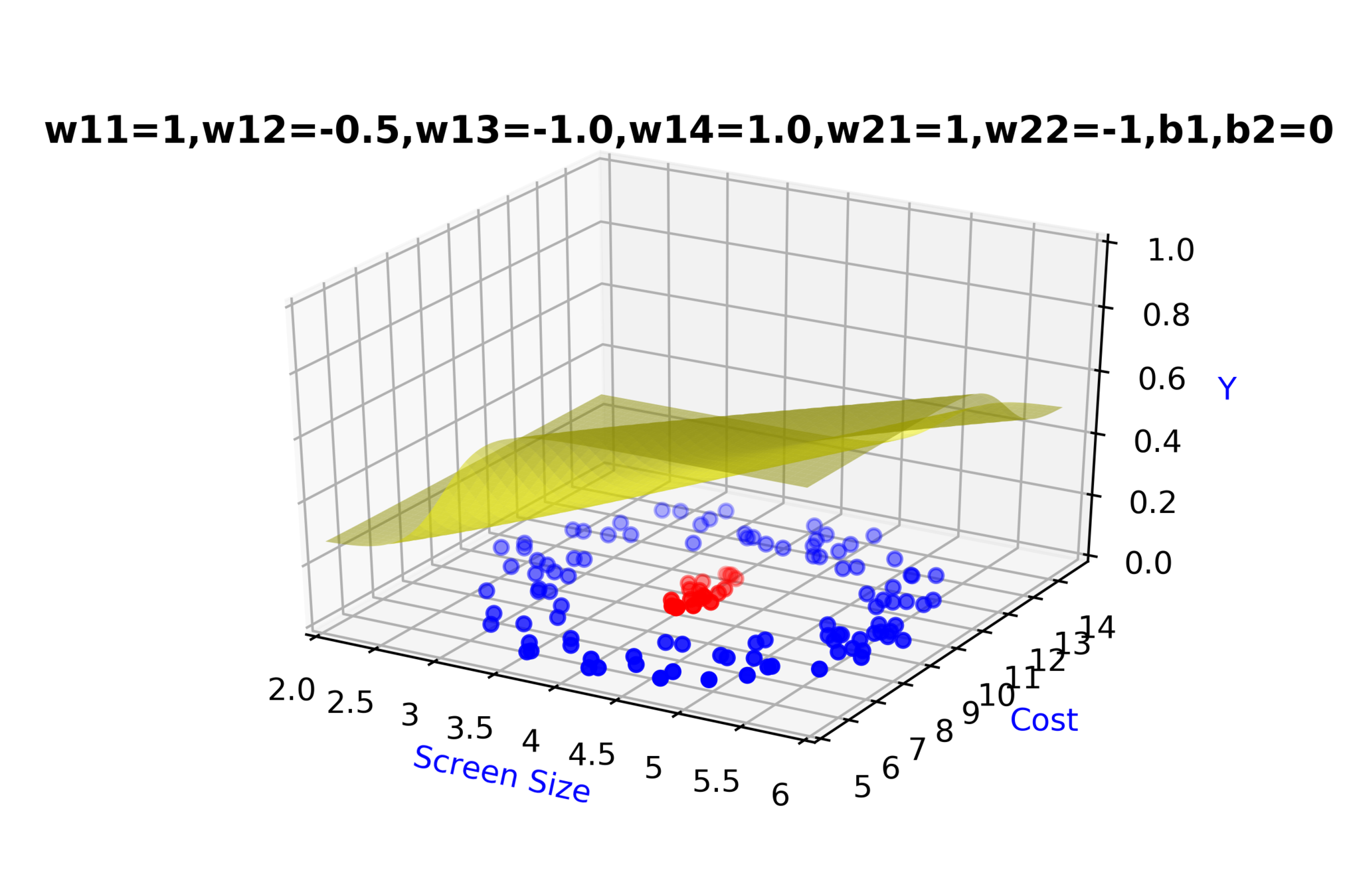
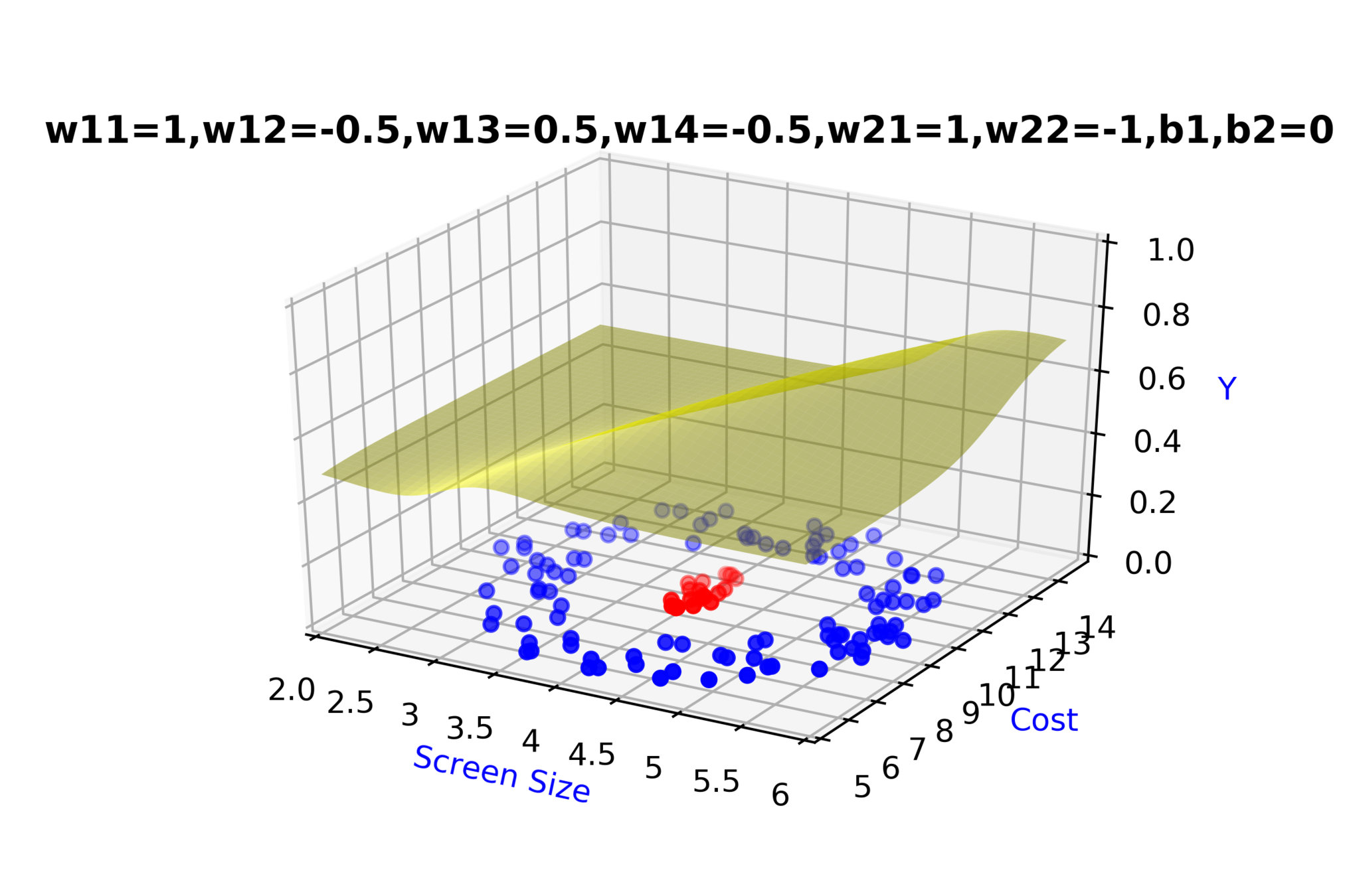
\( \hat{y} = g(h_1,h_2) \)

\(\hat{y} = \frac{1}{1+e^{-(w_{21}*h_1 + w_{22}*h_2 + b_2)}}\)
\(w_{14}\)

\(w_{13}\)

\(w_{22}\)

\( h_2 = f_2(x_1,x_2) \)

\( h_2 = \frac{1}{1+e^{-(w_{13}* x_1 + w_{14}*x_2+b_1)}} \)

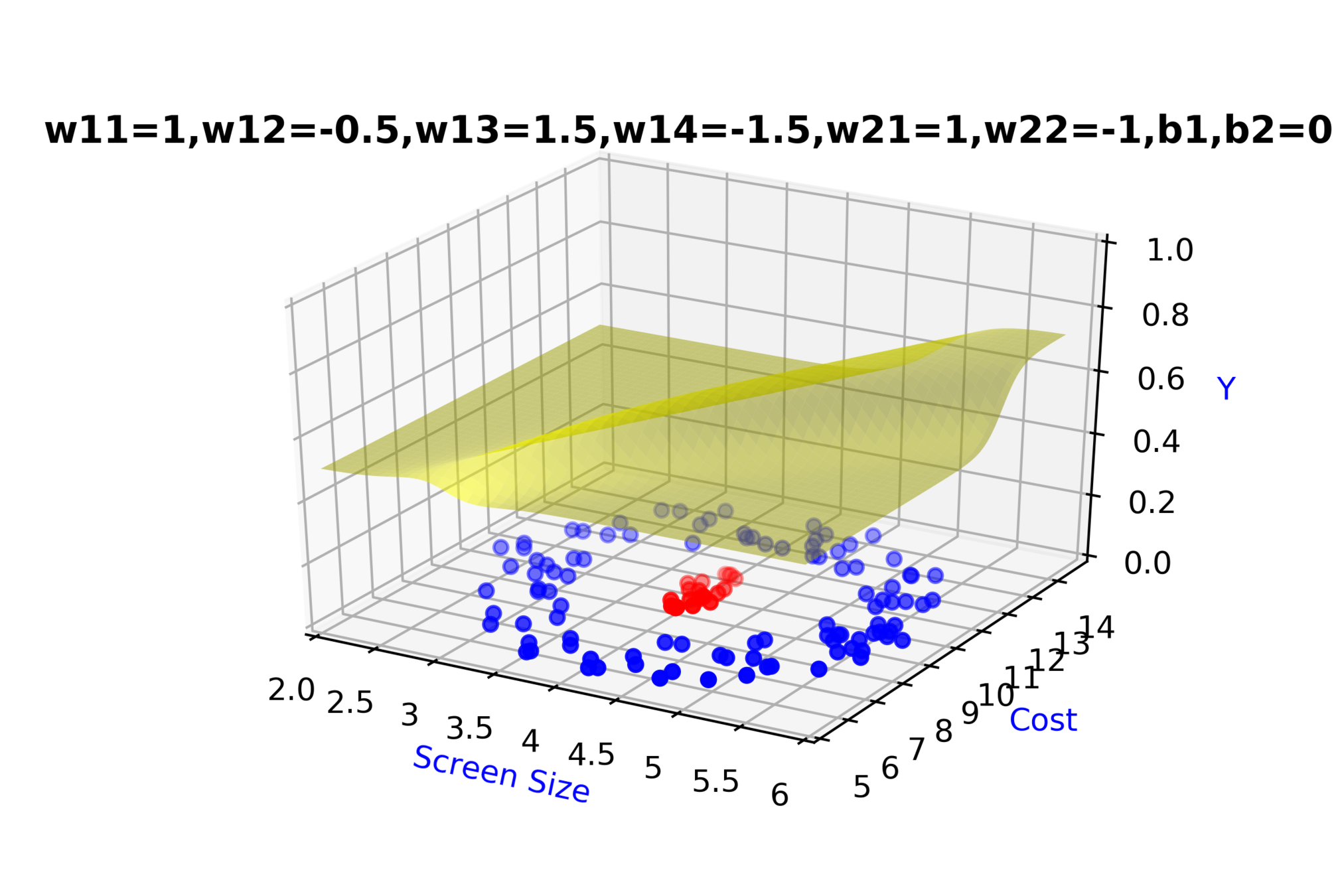
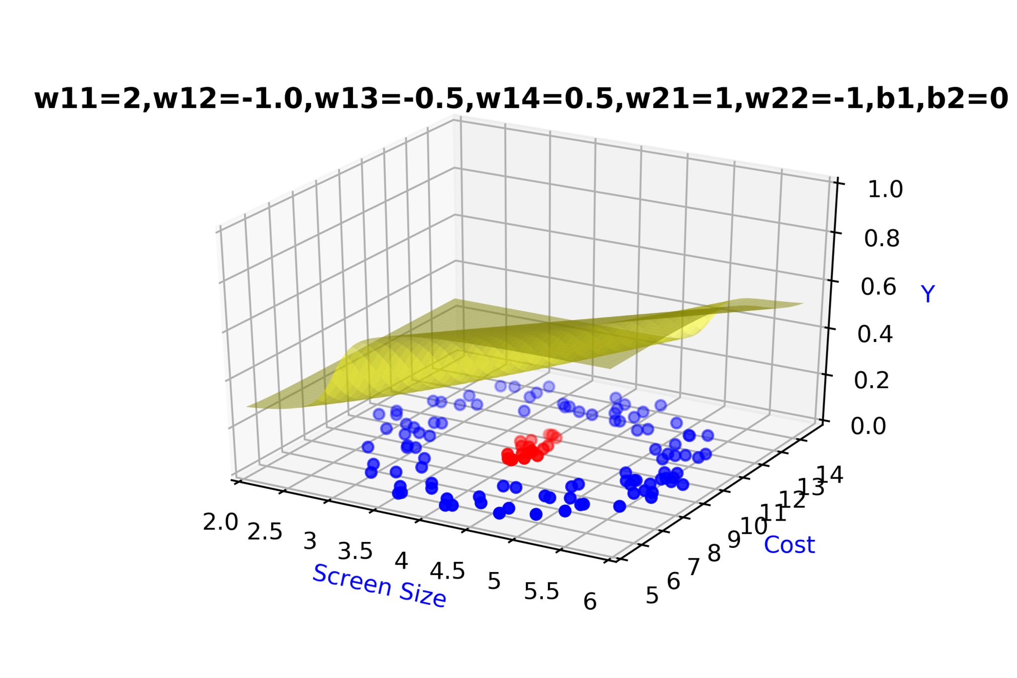
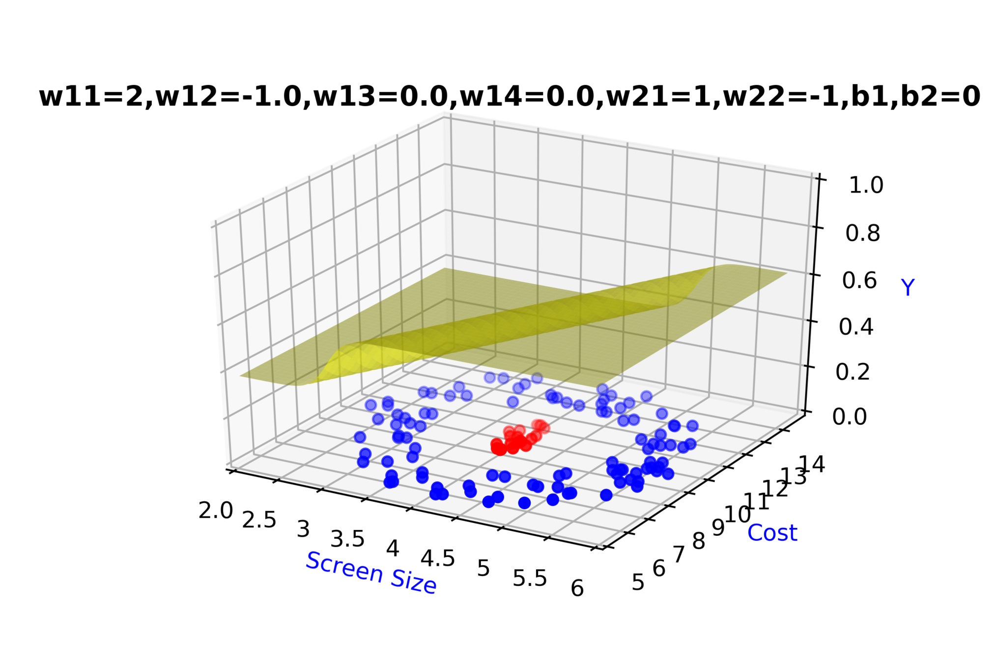
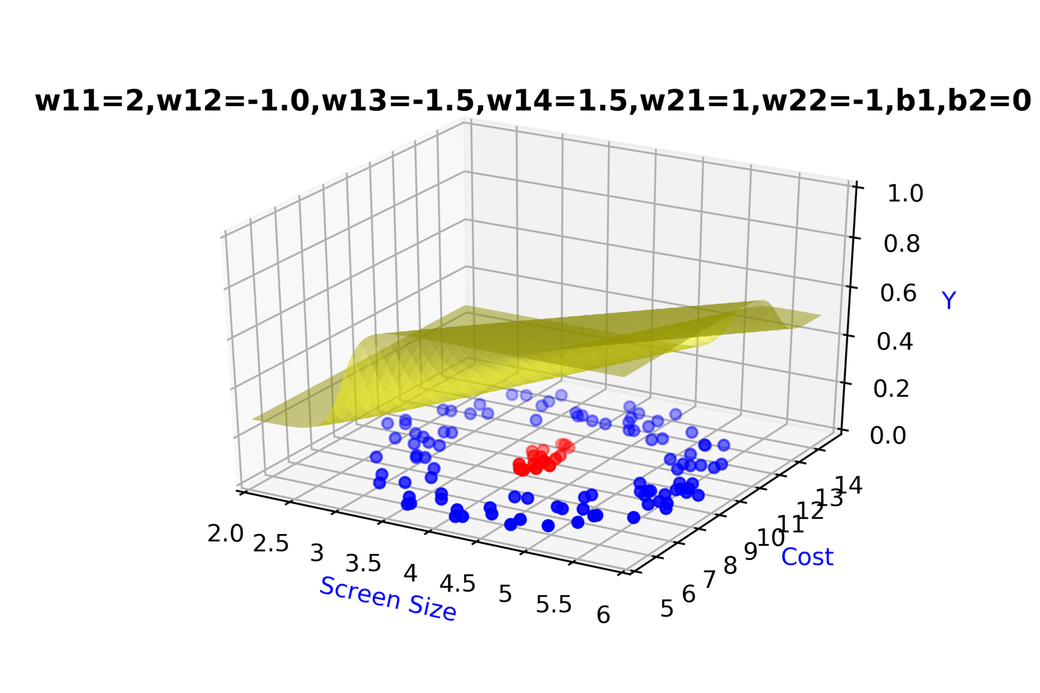
= \frac{1}{1+e^{-(w_{21}*(\frac{1}{1+e^{- (w_{11}*x_1 + w_{12}*x_2 + b_1)}}) + w_{22}*(\frac{1}{1+e^{- (w_{13}*x_1 + w_{14}*x_2 + b_1)}}) + b_2)}}

Model

Can we clarify the terminology a bit ?

(c) One Fourth Labs

x_2
W_3

\(h_{3} = \hat{y} = f(x) \)

x_3
W_1
b_1
W_2
b_2
b_3
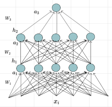
  • The pre-activation at layer 'i' is given by               

\( a_i(x) = W_ih_{i-1}(x) + b_i \)

  • The activation at layer 'i' is given by               

\( h_i(x) = g(a_i(x)) \)

a_1
h_1
a_2
h_2
a_3
  • The activation at output layer 'L' is given by               

\( f(x) = h_L =  O(a_L) \)

x_1

where 'g' is called as the activation function

where 'O' is called as the output activation function

(c) One Fourth Labs

x_1
x_2
W_3

\(h_{L} = \hat{y} = f(x) \)

x_3
W_1
b_1
W_2
b_2
b_3

\(\hat{y} = f(x) = O(W_3g(W_2g(W_1x + b_1) + b_2) + b_3)\) 

a_1
h_1
a_2
h_2
a_3

Model

How do we decide the output layer ?

Output\ Activation\ function\ is\ chosen\newline depending\ on\ the\ task\ at\ hand\newline (can\ be\ a\ softmax,\ linear)

Model

How do we decide the output layer ?

(c) One Fourth Labs

- On RHS show the imdb example from my lectures

- ON LHS show the apple example from my lecture

- Below LHS example, pictorially show other examples of regression from Kaggle 

- Below RHS example, pictorially show other examples of classification from Kaggle

- Finally show that in our contest also we need to do regression (bounding box predict x,y,w,h) and classification (character recognition)

Model

How do we decide the output layer ?

(c) One Fourth Labs

isActor

Damon

.  .  . 

isDirector

Nolan

.  .  .   .

\(x_i\)

imdb

Rating

critics

Rating

RT

Rating

\(y_i\) = {    8.8        7.3        8.1   846,320  }

\(y_i\) = {      1            0            0            0      }

x_1
x_2
x_3
x_4
x_5
W_1
W_2
W_3
a_1
h_1
a_2
h_2
a_3

Apple

Banana

Orange

Grape

W_1
W_2
W_3
a_1
h_1
a_2
h_2
a_3
b_1
b_2
b_1
b_2
b_3
b_3

Box Office

Collection

Model

What is the output layer for regression problems ?

(c) One Fourth Labs


x = [x1, x2, x3, x4, x5]

def sigmoid(a):
    return 1.0/(1.0+ np.exp(-a))


def output_layer(a):
    return a


def forward_propagation(x): 
    L = 3  #Total number of layers 
    W = {...} #Assume weights are learnt

    a[1] = W[1]*x + b[1]    

    for i in range(1,L):
        h[i] = sigmoid(a[i])
        a[i+1] = W[i+1]*h[i] + b[i+1]
    
    Y = output_layer(a[L])
    
x_1
x_2
x_3
x_4
x_5
W_1
W_2
W_3
a_1
h_1
a_2
h_2
a_3
b_1
b_2
b_3

Model

What is the output layer for classification problems ?

(c) One Fourth Labs

x_1
x_1
x_2
x_3
x_4
x_5
W_1
W_2
W_3
a_1
h_1
a_2
h_2
a_3

Apple

\(\hat{y}\) = {  1,  0,  0,  0  }

Banana

Orange

Grape

True Output :

\(\hat{y}\) = {  0.64,  0.03,  0.26,  0.07  }

Predicted Output :

What kind of output activation function should we use?

Model

What is the output layer for classification problems ?

x_2
.
.
.
x_{99}
W_1
W_2
W_3
a_1
h_1
a_2
h_2
a_3

Apple

Banana

Orange

Grape

W_1 = \begin{bmatrix} w_{1\ 1\ 1} & w_{1\ 1\ 2} & . & . & . & w_{1\ 1\ 99} & w_{1\ 1\ 100} \\ w_{1\ 2\ 1} & w_{1\ 2\ 2} & . & . & . & w_{1\ 2\ 99} & w_{1\ 2\ 100} \\ . & . & . & . & . & . & .\\ . & . & . & . & . & . & .\\ w_{1\ 10\ 1} & w_{1\ 10\ 2} & . & . & . & w_{1\ 10\ 99} & w_{1\ 10\ 100} \\ \end{bmatrix}
a_{1\ 1} = w_{1\ 1\ 1}*x_1 + w_{1\ 1\ 2}*x_2 + w_{1\ 1\ 3}*x_3 + .... + w_{1\ 1\ 100}*x_{100}
a_{1\ 2} = w_{1\ 2\ 1}*x_1 + w_{1\ 2\ 2}*x_2 + w_{1\ 2\ 3}*x_3 + .... + w_{1\ 2\ 100}*x_{100}

.

a_{1\ 10} = w_{1\ 10\ 1}*x_1 + w_{1\ 10\ 2}*x_2 + w_{1\ 10\ 3}*x_3 + .... + w_{1\ 10\ 100}*x_{100}

.

.

.

.

.

\(a_1 = W_1*x\)

X = \begin{bmatrix} x_{1} \\ x_{2} \\ . \\ . \\ x_{100} \\ \end{bmatrix}
x_1
x_{100}

Model

What is the output layer for classification problems ?

\(a_1 = W_1*x\)

\(h_{11} = g(a_{11})\)

\(h_{12} = g(a_{12})\)

\(h_{1\ 10} = g(a_{1\ 10})\)

.      .      .       .

x_2
.
.
.
x_{99}
W_1
W_2
W_3
a_1
h_1
a_2
h_2
a_3

Apple

Banana

Orange

Grape

x_1
x_{100}
W_1 = \begin{bmatrix} w_{1\ 1\ 1} & w_{1\ 1\ 2} & . & . & . & w_{1\ 1\ 99} & w_{1\ 1\ 100} \\ w_{1\ 2\ 1} & w_{1\ 2\ 2} & . & . & . & w_{1\ 2\ 99} & w_{1\ 2\ 100} \\ . & . & . & . & . & . & .\\ . & . & . & . & . & . & .\\ w_{1\ 10\ 1} & w_{1\ 10\ 2} & . & . & . & w_{1\ 10\ 99} & w_{1\ 10\ 100} \\ \end{bmatrix}
X = \begin{bmatrix} x_{1} \\ x_{2} \\ . \\ . \\ x_{100} \\ \end{bmatrix}

\(h_1 = g(a_1)\)

Model

What is the output layer for classification problems ?

(c) One Fourth Labs

W_2 = \begin{bmatrix} w_{2\ 1\ 1} & w_{2\ 1\ 2} & . & . & . & w_{2\ 1\ 10} \\ w_{2\ 2\ 1} & w_{2\ 2\ 2} & . & . & . & w_{2\ 2\ 10} \\ . & . & . & . & . & . \\ . & . & . & . & . & . \\ w_{2\ 10\ 1} & w_{2\ 10\ 2} & . & . & . & w_{2\ 10\ 10} \\ \end{bmatrix}
a_{2\ 1} = w_{2\ 1\ 1}*h_{1\ 1} + w_{2\ 1\ 2}*h_{1\ 2} + w_{2\ 1\ 3}*h_{1\ 3} + .... + w_{2\ 1\ 10}*h_{1\ 10}
a_{2\ 2} = w_{2\ 2\ 1}*h_{1\ 1} + w_{2\ 2\ 2}*h_{1\ 2} + w_{2\ 2\ 3}*h_{1\ 3} + .... + w_{2\ 2\ 10}*h_{1\ 10}
a_{2\ 10} = w_{2\ 10\ 1}*h_{1\ 1} + w_{2\ 10\ 2}*h_{1\ 2} + w_{2\ 10\ 3}*h_{1\ 3} + .... + w_{2\ 10\ 10}*h_{1\ 10}
x_2
.
.
.
x_{99}
W_1
W_2
W_3
a_1
h_1
a_2
h_2
a_3

Apple

Banana

Orange

Grape

x_1
x_{100}
h_{1} = \begin{bmatrix} h_{1\ 11} \\ h_{1\ 2} \\ . \\ . \\ h_{1\ 10} \\ \end{bmatrix}

.

.

.

.

.

.

\(a_2 = W_2*h_1\)

Model

What is the output layer for classification problems ?

(c) One Fourth Labs

\(a_2 = W_2*h_1\)

\(h_{21} = g(a_{21})\)

\(h_{22} = g(a_{22})\)

\(h_{2\ 10} = g(a_{2\ 10})\)

.      .      .       .

W_2 = \begin{bmatrix} w_{2\ 1\ 1} & w_{2\ 1\ 2} & . & . & . & w_{2\ 1\ 10} \\ w_{2\ 2\ 1} & w_{2\ 2\ 2} & . & . & . & w_{2\ 2\ 10} \\ . & . & . & . & . & . \\ . & . & . & . & . & . \\ w_{2\ 10\ 1} & w_{2\ 10\ 2} & . & . & . & w_{2\ 10\ 10} \\ \end{bmatrix}
h_{1} = \begin{bmatrix} h_{1\ 11} \\ h_{1\ 2} \\ . \\ . \\ h_{1\ 10} \\ \end{bmatrix}
x_2
.
.
.
x_{99}
W_1
W_2
W_3
a_1
h_1
a_2
h_2
a_3

Apple

Banana

Orange

Grape

x_1
x_{100}

\(h_2 = g(a_2)\)

Model

What is the output layer for classification problems ?

W_3 = \begin{bmatrix} w_{3\ 1\ 1} & w_{3\ 1\ 2} & . & . & . & w_{3\ 1\ 10} \\ w_{3\ 2\ 1} & w_{3\ 2\ 2} & . & . & . & w_{3\ 2\ 10} \\ w_{3\ 3\ 1} & w_{3\ 3\ 2} & . & . & . & w_{3\ 3\ 10} \\ w_{3\ 4\ 1} & w_{3\ 4\ 2} & . & . & . & w_{3\ 4\ 10} \\ \end{bmatrix}
a_{3\ 1} = w_{3\ 1\ 1}*h_{2\ 1} + w_{3\ 1\ 2}*h_{2\ 2} + w_{3\ 1\ 3}*h_{2\ 3} + .... + w_{3\ 1\ 10}*h_{2\ 10}
a_{3\ 2} = w_{3\ 2\ 1}*h_{2\ 1} + w_{3\ 2\ 2}*h_{2\ 2} + w_{3\ 2\ 3}*h_{2\ 3} + .... + w_{3\ 2\ 10}*h_{2\ 10}
a_{3\ 4} = w_{3\ 4\ 1}*h_{2\ 1} + w_{3\ 4\ 2}*h_{2\ 2} + w_{3\ 4\ 3}*h_{2\ 3} + .... + w_{3\ 4\ 10}*h_{2\ 10}
h_{2} = \begin{bmatrix} h_{2\ 1} \\ h_{2\ 2} \\ . \\ . \\ h_{2\ 10} \\ \end{bmatrix}
a_{3\ 3} = w_{3\ 3\ 1}*h_{2\ 1} + w_{3\ 3\ 2}*h_{2\ 2} + w_{3\ 3\ 3}*h_{2\ 3} + .... + w_{3\ 3\ 10}*h_{2\ 10}
x_2
.
.
.
x_{99}
W_1
W_2
W_3
a_1
h_1
a_2
h_2
a_3

Apple

Banana

Orange

Grape

x_1
x_{100}

\(a_3 = W_3*h_2\)

Model

What is the output layer for classification problems ?

\(a_3 = W_3*h_2\)

\(\hat{y}_{1} = O(a_{31})\)

\(\hat{y}_{2} = O(a_{32})\)

\(\hat{y}_{4} = O(a_{34})\)

\(\hat{y}_{3} = O(a_{33})\)

x_2
.
.
.
x_{99}
W_1
W_2
W_3
a_1
h_1
a_2
h_2
a_3

Apple

Banana

Orange

Grape

x_1
x_{100}
W_3 = \begin{bmatrix} w_{3\ 1\ 1} & w_{3\ 1\ 2} & . & . & . & w_{3\ 1\ 10} \\ w_{3\ 2\ 1} & w_{3\ 2\ 2} & . & . & . & w_{3\ 2\ 10} \\ w_{3\ 3\ 1} & w_{3\ 3\ 2} & . & . & . & w_{3\ 3\ 10} \\ w_{3\ 4\ 1} & w_{3\ 4\ 2} & . & . & . & w_{3\ 4\ 10} \\ \end{bmatrix}
h_{2} = \begin{bmatrix} h_{2\ 1} \\ h_{2\ 2} \\ . \\ . \\ h_{2\ 10} \\ \end{bmatrix}

Model

What is the output layer for classification problems ?

(c) One Fourth Labs

Take each entry and divide by the sum of all entries

\hat{y}_{1} = \cfrac{3}{(3+4+10+3)} = 0.15
\hat{y}_{2} = \cfrac{4}{(3+4+10+3)} = 0.20
\hat{y}_{3} = \cfrac{10}{(3+4+10+3)} = 0.50
\hat{y}_{4} = \cfrac{3}{(3+4+10+3)} = 0.15
\hat{y}_{1} = \cfrac{7}{(7+(-2)+4+1)} = 0.70
\hat{y}_{2} = \cfrac{-2}{(7+(-2)+4+1)} = -0.20
Say \ a_3 = [\ 3\ \ 4\ \ 10\ \ 3\ ]
Say \ for \ other \ input \ a_3 = [\ 7\ \ -2\ \ 4\ \ 1\ ]
\hat{y}_{3} = \cfrac{4}{(7+(-2)+4+1)} = 0.40
\hat{y}_{4} = \cfrac{1}{(7+(-2)+4+1)} = 0.10

We will now try using softmax function

x_2
.
.
.
x_{99}
W_1
W_2
W_3
a_1
h_1
a_2
h_2
a_3

Apple

Banana

Orange

Grape

x_1
x_{100}
Output\ Activation\ Function\ has\ to\ be\ chosen\newline such\ that\ output\ is\ probability

Model

What is the output layer for classification problems ?

(c) One Fourth Labs

softmax(z_{i}) =\cfrac{e^{z_{i}}}{\displaystyle\sum_{j=1}^{k}e^{z_{j}}} \ \ for \ i= 1.....k
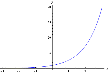
y =e^x
e^x\ \ is \ \ positive \ \ even \ \ for \ \ negative \ \ values \ \ of \ \ x

Model

What is the output layer for classification problems ?

(c) One Fourth Labs

\(h = [   h_{1}    h_{2}      h_{3}     h_{4}    ]\)

\(softmax(h) = [softmax(h_{1})      softmax(h_{2})        softmax(h_{3})     softmax(h_{4})] \)

softmax(h) = \begin{bmatrix} \cfrac{e^{h_{1}}}{\displaystyle\sum_{j=1}^{4}e^{h_{j}}} \ \ & \cfrac{e^{h_{2}}}{\displaystyle\sum_{j=1}^{4}e^{h_{j}}} \ \ & \cfrac{e^{h_{3}}}{\displaystyle\sum_{j=1}^{4}e^{h_{j}}} \ \ & \cfrac{e^{h_{4}}}{\displaystyle\sum_{j=1}^{4}e^{h_{j}}} \\ \end{bmatrix}
x_2
.
.
.
x_{99}
W_1
W_2
W_3
a_1
h_1
a_2
h_2
a_3

Apple

Banana

Orange

Grape

x_1
x_{100}
softmax(h_{i})\ is\ the\ i^{th}\ element\newline of\ softmax\ output

Model

What is the output layer for classification problems ?

(c) One Fourth Labs

x_2
.
.
.
x_{99}
W_1
W_2
W_3
a_1
h_1
a_2
h_2
a_3

Apple

Banana

Orange

Grape

x_1
x_{100}

\(a_2 = W_2*h_1\)

\(h_2 = g(a_2)\)

\(a_1 = W_1*x\)

\(a_3 = W_3*h_2\)

\(h_1 = g(a_1)\)

\(\hat{y} = softmax(a_3)\)

Model

What is the output layer for regression problems ?

isActor

Damon

.  .  . 

isDirector

Nolan

.  .  .   .

\(x_i\)

W_1
W_2
W_3
a_1
h_1
a_2
h_2
a_3

Box Office

Collection

\(\hat{y}\) = $ 15,032,493.29

True Output :

\(\hat{y}\) = $  10,517,330.07

Predicted Output :

What kind of output function should we use?

Model

W_1
W_2
W_3
a_1
h_1
a_2
h_2
a_3
W_1 = \begin{bmatrix} w^{1}_{1\ 1} & w_{1\ 1\ 2} & . & . & . & w_{1\ 1\ 9} & w_{1\ 1\ 10} \\ w_{1\ 2\ 1} & w_{1\ 2\ 2} & . & . & . & w_{1\ 2\ 9} & w_{1\ 2\ 10} \\ . & . & . & . & . & . & .\\ . & . & . & . & . & . & .\\ w_{1\ 5\ 1} & w_{1\ 5\ 2} & . & . & . & w_{1\ 5\ 9} & w_{1\ 5\ 10} \\ \end{bmatrix}
a_{1\ 1} = w_{1\ 1\ 1}*x_1 + w_{1\ 1\ 2}*x_2 + w_{1\ 1\ 3}*x_3 + .... + w_{1\ 1\ 10}*x_{10}
a_{1\ 2} = w_{1\ 2\ 1}*x_1 + w_{1\ 2\ 2}*x_2 + w_{1\ 2\ 3}*x_3 + .... + w_{1\ 2\ 10}*x_{10}

.

a_{1\ 5} = w_{1\ 5\ 1}*x_1 + w_{1\ 5\ 2}*x_2 + w_{1\ 5\ 3}*x_3 + .... + w_{1\ 5\ 10}*x_{10}

.

.

.

.

.

\(a_1 = W_1*x\)

X = \begin{bmatrix} x_{1} \\ x_{2} \\ . \\ . \\ x_{10} \\ \end{bmatrix}

What is the output layer for regression problems ?

Box Office

Collection

isActor

Damon

.     .      .

isDirector

Nolan

 .     .      .

\(x_i\)

Model

\(a_1 = W_1*x\)

\(h_{11} = g(a_{11})\)

\(h_{12} = g(a_{12})\)

\(h_{1\ 5} = g(a_{1\ 5})\)

.      .      .       .

\(h_1 = g(a_1)\)

W_1
W_2
W_3
a_1
h_1
a_2
h_2
a_3

Box Office

Collection

isActor

Damon

.     .      .

isDirector

Nolan

 .     .      .

\(x_i\)

W_1 = \begin{bmatrix} w_{1\ 1\ 1} & w_{1\ 1\ 2} & . & . & . & w_{1\ 1\ 9} & w_{1\ 1\ 10} \\ w_{1\ 2\ 1} & w_{1\ 2\ 2} & . & . & . & w_{1\ 2\ 9} & w_{1\ 2\ 10} \\ . & . & . & . & . & . & .\\ . & . & . & . & . & . & .\\ w_{1\ 5\ 1} & w_{1\ 5\ 2} & . & . & . & w_{1\ 5\ 9} & w_{1\ 5\ 10} \\ \end{bmatrix}
X = \begin{bmatrix} x_{1} \\ x_{2} \\ . \\ . \\ x_{10} \\ \end{bmatrix}

What is the output layer for regression problems ?

Model

W_2 = \begin{bmatrix} w_{2\ 1\ 1} & w_{2\ 1\ 2} & . & . & . & w_{2\ 1\ 5} \\ w_{2\ 2\ 1} & w_{2\ 2\ 2} & . & . & . & w_{2\ 2\ 5} \\ . & . & . & . & . & . \\ . & . & . & . & . & . \\ w_{2\ 5\ 1} & w_{2\ 5\ 2} & . & . & . & w_{2\ 5\ 5} \\ \end{bmatrix}
a_{2\ 1} = w_{2\ 1\ 1}*h_{1\ 1} + w_{2\ 1\ 2}*h_{1\ 2} + w_{2\ 1\ 3}*h_{1\ 3} + .... + w_{2\ 1\ 5}*h_{1\ 5}
a_{2\ 2} = w_{2\ 2\ 1}*h_{1\ 1} + w_{2\ 2\ 2}*h_{1\ 2} + w_{2\ 2\ 3}*h_{1\ 3} + .... + w_{2\ 2\ 5}*h_{1\ 5}
a_{2\ 5} = w_{2\ 5\ 1}*h_{1\ 1} + w_{2\ 5\ 2}*h_{1\ 2} + w_{2\ 5\ 3}*h_{1\ 3} + .... + w_{2\ 5\ 5}*h_{1\ 5}
h_{1} = \begin{bmatrix} h_{1\ 1} \\ h_{1\ 2} \\ . \\ . \\ h_{1\ 5} \\ \end{bmatrix}

.

.

.

.

.

.

\(a_2 = W_2*h_1\)

W_1
W_2
W_3
a_1
h_1
a_2
h_2
a_3

Box Office

Collection

isActor

Damon

.     .      .

isDirector

Nolan

 .     .      .

\(x_i\)

What is the output layer for regression problems ?

Model

\(a_2 = W_2*h_1\)

\(h_{21} = g(a_{21})\)

\(h_{22} = g(a_{22})\)

\(h_{2\ 5} = g(a_{2\ 5})\)

.      .      .       .

\(h_2 = g(a_2)\)

h_{1} = \begin{bmatrix} h_{1\ 1} \\ h_{1\ 2} \\ . \\ . \\ h_{1\ 5} \\ \end{bmatrix}
W_2 = \begin{bmatrix} w_{2\ 1\ 1} & w_{2\ 1\ 2} & . & . & . & w_{2\ 1\ 5} \\ w_{2\ 2\ 1} & w_{2\ 2\ 2} & . & . & . & w_{2\ 2\ 5} \\ . & . & . & . & . & . \\ . & . & . & . & . & . \\ w_{2\ 5\ 1} & w_{2\ 5\ 2} & . & . & . & w_{2\ 5\ 5} \\ \end{bmatrix}
W_1
W_2
W_3
a_1
h_1
a_2
h_2
a_3

Box Office

Collection

isActor

Damon

.     .      .

isDirector

Nolan

 .     .      .

\(x_i\)

What is the output layer for regression problems ?

Model

W_3 = \begin{bmatrix} w_{3\ 1} & w_{3\ 2} & . & . & . & w_{3\ 5} \\ \end{bmatrix}
a_{3} = w_{3\ 1}*h_{2\ 1} + w_{3\ 2}*h_{2\ 2} + w_{3\ 3}*h_{2\ 3} + .... + w_{3\ 5}*h_{2\ 5}
h_{2} = \begin{bmatrix} h_{2\ 1} \\ h_{2\ 2} \\ . \\ . \\ h_{2\ 5} \\ \end{bmatrix}

\(a_3 = W_3*h_2\)

W_1
W_2
W_3
a_1
h_1
a_2
h_2
a_3

Box Office

Collection

isActor

Damon

.     .      .

isDirector

Nolan

 .     .      .

\(x_i\)

\(\hat{y} = O(a_{3})\)

What is the output layer for regression problems ?

Model

Can we use sigmoid function ?

Say \ a_3 = [\ 2500.03\ ]

NO

What is the output layer for regression problems ?

Can we use softmax function ?

NO

Can we use real numbered pre-activation as it is ?

Yes, it is a real number after all

What happens if we get a negative output ?

Should we not normalize it ?

W_1
W_2
W_3
a_1
h_1
a_2
h_2
a_3

Box Office

Collection

isActor

Damon

.     .      .

isDirector

Nolan

 .     .      .

\(x_i\)

Output\ Activation\ Function\ has\ to\ be\ chosen\newline such\ that\ output\ is\ real\ number

Model

(c) One Fourth Labs

\(a_2 = W_2*h_1\)

\(h_2 = g(a_2)\)

\(a_1 = W_1*x\)

\(a_3 = W_3*h_2\)

\(h_1 = g(a_1)\)

\(\hat{y} = a_3\)

What is the output layer for regression problems ?

W_1
W_2
W_3
a_1
h_1
a_2
h_2
a_3

Box Office

Collection

isActor

Damon

.     .      .

isDirector

Nolan

 .     .      .

\(x_i\)

Model

Can we see the model in action?

(c) One Fourth Labs

1) We will show the demo which Ganga is preparing

Model

In practice how would you deal with extreme non-linearity ?

(c) One Fourth Labs

x_{1}
x_{2}

-

-

-

-

-

-

x_{3}

-

-

-

x_{4}

-

-

-

Model

In practice how would you deal with extreme non-linearity ?

(c) One Fourth Labs

\(Model\)

\(Loss\)

Model

Why is Deep Learning also called Deep Representation Learning ?

(c) One Fourth Labs

x_2
.
.
.
W_{L-1}
W_L
h_{L-2}
a_{L-1}
a_L

Apple

Banana

Orange

Grape

x_1
x_{N*N}
N\ X\ N \ image
.
.
.
.
.
.
.
.
.
.
.
.
.
.
.
.
.
.
.
.
.
.
.
.
.
.
.
.
.
.
.
.
.
.
.
.
.
h_{L-1}
In\ addition\ to\ predicting\ output,\ we\ are\ also\ learning\newline the\ intermediate\ representations\ which\ help\ us\ in\newline predicting\ the\ output\ better

Loss Function

What is the loss function that you use for a regression problem ?

(c) One Fourth Labs

 Size in feet^2  No of bedrroms House Rent (Rupees) in 1000's
850 2 12
1100 2 20
1000 3 19
.... .... ....
x_1
x_2
b_1
b_2

\(h_{2} = \hat{y} = f(x) \)

W_2
W_1
a_1
h_1
a_2
W_2 = [\ \ 100 \ \ \ \ 100\ \ ]
b = [\ \ 0\ \ \ \ 0.9\ \ ]

\(a_1    =    W_1*x + b_1      =      [   0.67       -0.415   ]\) 

\(h_1   =   sigmoid(a_1)    =     [   0.66         0.40   ]\)

\(a_2    =    W_2*h_1 + b_2   =     11.5 \)

\(h_2    =    a_2        =        11.5\)

Output :

Squared Error Loss :

L(\Theta) = \frac{1}{N} \displaystyle\sum_{i=1}^N \displaystyle\sum_{i=1}^d (\hat{y}_{ij} - y_{ij})^2

\(L(\Theta) = (11.5 - 12)^2\)


\(= (0.25)\)


W_1 = \begin{bmatrix} 0.0002 & 0.25 \\ 0.0001 & -0.25 \\ \end{bmatrix}

Loss Function

What is the loss function that you use for a regression problem ?

(c) One Fourth Labs

 Size in feet^2   No of bedrroms House Rent (Rupees) in 1000's
850 2 12
1100 2 14
1000 3 15
.... .... ....
x_1
x_2
b_1
b_2

\(h_{2} = \hat{y} = f(x) \)

W_2
W_1
a_1
h_1
a_2

\(a_1    =    W_1*x + b_1    =    [   0.72         -0.39   ]\)

\(h_1    =   sigmoid(a_1)   =    [   0.67         0.40   ]\)

\(a_2    =    W_2*h_1 + b_2  =     11.6 \)

\(h_2    =    a_2        =     11.6\)

Output :

Squared Error Loss :

L(\Theta) = \frac{1}{N} \displaystyle\sum_{i=1}^N \displaystyle\sum_{i=1}^d (\hat{y}_{ij} - y_{ij})^2

\(L(\Theta) = (11.6 - 14)^2\)


\(= (5.76)\)


W_2 = [\ \ 100 \ \ \ \ 100\ \ ]
b = [\ \ 0\ \ \ \ 0.9\ \ ]
W_1 = \begin{bmatrix} 0.0002 & 0.25 \\ 0.0001 & -0.25 \\ \end{bmatrix}

Loss Function

What is the loss function that you use for a regression problem ?

(c) One Fourth Labs

 Size in feet^2   No of bedrroms House Rent (Rupees) in 1000's
850 2 12
1100 2 14
1000 3 15
.... .... ....
x_1
x_2
b_1
b_2

\(h_{2} = \hat{y} = f(x) \)

W_2
W_1
a_1
h_1
a_2

\(a_1    =      W_1*x + b_1        =   [   0.95         -0.65   ]\)

\(h_1    =    sigmoid(a_1)        =   [   0.72          0.34   ]\)

\(a_2    =    W_2*h_1 + b_2     =    11.5 \)

\(h_2    =   a_2         =    11.5\)

Output :

Squared Error Loss :

L(\Theta) = \frac{1}{N} \displaystyle\sum_{i=1}^N \displaystyle\sum_{i=1}^d (\hat{y}_{ij} - y_{ij})^2

\(L(\Theta) = (11.5 - 15)^2\)


\(= (12.25)\)

W_2 = [\ \ 100 \ \ \ \ 100\ \ ]
b = [\ \ 0\ \ \ \ 0.9\ \ ]
W_1 = \begin{bmatrix} 0.0002 & 0.25 \\ 0.0001 & -0.25 \\ \end{bmatrix}

Loss Function

What is the loss function that you use for a regression problem ?

(c) One Fourth Labs

 Size in feet^2   No of bedrroms House Rent (Rupees) in 1000's
850 2 12
1100 2 14
1000 3 15
.... .... ....
x_1
x_2
b_1
b_2

\(h_{2} = \hat{y} = f(x) \)

W_2
W_1
a_1
h_1
a_2
W_2 = [\ \ 100 \ \ \ \ 100\ \ ]
b = [\ \ 0\ \ \ \ 0.9\ \ ]
W_1 = \begin{bmatrix} 0.0002 & 0.25 \\ 0.0001 & -0.25 \\ \end{bmatrix}

X = [X1, X2, X3, X4, ..., XN] #N 'd' dimensiomal data points
Y = [y1, y2, y3, y4, ..., yN]


def sigmoid(a):
    return 1.0/(1.0+ np.exp(-a))


def output_layer(a):
    return a


def forward_propagation(X): 
    L = 3  #Total number of layers 
    W = {...} #Assume weights are learnt

    a[1] = W[1]*X + b[1]    

    for i in range(1,L):
        h[i] = sigmoid(a[i])
        a[i+1] = W[i+1]*h[i] + b[i+1]
    
    return output_layer(a[L])
    
    
def compute_loss(X,Y):
    N = len(X) #Number of data points

    loss = 0
    for x,y in zip(X,Y):
        fx = forward_propagation(X)
        loss += (1/N)*(fx - y)**2

    return loss
    

Loss Function

W_1 = \begin{bmatrix} 0.9 & 0.2 & 0.4 & 0.3 \\ -0.5 & 0.4 & 0.3 & 0.3 \\ 0.1 & 0.1 & -0.1 & 0.2 \\ -0.2 & 0.5 & 0.5 & 0.7 \\ \end{bmatrix}

\(x_i\)

W_1
W_2
b_1
b_2
W_2 = \begin{bmatrix} 0.5 & 0.8 & -0.6 & 0.3 \\ \end{bmatrix}
y = 1
x = [\ \ 0.3\ \ \ 0.5 \ \ \ -0.4 \ \ \ 0.3\ \ ]

\(a_1   =   W_1*x + b_1      =   [   0.8      0.52      0.68         0.7   ]\) 

\(h_1   =   sigmoid(a_1)   =   [   0.69       0.63       0.66       0.67   ]\)

\(a_2   =   W_2*h_1 + b_2   =   0.948\)

\(\hat{y}   =   sigmoid(a_2)   =   0.7207\)

Output :

a_1
h_1
b = [\ \ 0.5\ \ \ 0.3\ \ ]

Cross Entropy Loss:

L(\Theta) = \frac{1}{N} \displaystyle\sum_{i=1}^N \begin{cases} -log{(\hat{y})} &\text{if } y = 1 \\ -log{(1 - \hat{y})} &\text{if } y = 0 \end{cases}

\(L(\Theta) = -1*\log({0.7207})\)

\(= 0.327\)

a_2

What is the loss function that you use for a binary classification problem ?

Loss Function

\(x_i\)

W_1
W_2
b_1
b_2
W_2 = \begin{bmatrix} 0.5 & 0.8 & -0.6 & 0.3 \\ \end{bmatrix}
y = 0
x = [\ \ -0.6\ \ \ -0.6 \ \ \ 0.2 \ \ \ 0.3\ \ ]

\(a_1   =   W_1*x + b_1      =   [   0.01       0.71      0.42         0.63  ]\) 

\(h_1   =   sigmoid(a_1)    =   [   0.50       0.67       0.60       0.65   ]\)

\(a_2   =   W_2*h_1 + b_2   =   0.921\)

\(\hat{y}   =   sigmoid(a_2)   =   0.7152\)

Output :

a_1
h_1
b = [\ \ 0.5\ \ \ 0.3\ \ ]

Cross Entropy Loss:

L(\Theta) = \frac{1}{N} \displaystyle\sum_{i=1}^N \begin{cases} -log{(\hat{y})} &\text{if } y = 1 \\ -log{(1 - \hat{y})} &\text{if } y = 0 \end{cases}

\(L(\Theta) = -1*\log({1- 0.7152})\)

a_2

\(= 1.2560\)

What is the loss function that you use for a binary classification problem ?

W_1 = \begin{bmatrix} 0.9 & 0.2 & 0.4 & 0.3 \\ -0.5 & 0.4 & 0.3 & 0.3 \\ 0.1 & 0.1 & -0.1 & 0.2 \\ -0.2 & 0.5 & 0.5 & 0.7 \\ \end{bmatrix}

Loss Function

\(x_i\)

W_1
W_2
b_1
b_2
W_2 = \begin{bmatrix} 0.5 & 0.8 & -0.6 & 0.3 \\ \end{bmatrix}
a_1
h_1
b = [\ \ 0.5\ \ \ 0.3\ \ ]
a_2

What is the loss function that you use for a binary classification problem ?

W_1 = \begin{bmatrix} 0.9 & 0.2 & 0.4 & 0.3 \\ -0.5 & 0.4 & 0.3 & 0.3 \\ 0.1 & 0.1 & -0.1 & 0.2 \\ -0.2 & 0.5 & 0.5 & 0.7 \\ \end{bmatrix}

X = [X1, X2, X3, X4, ..., XN] #N 'd' dimensiomal data points
Y = [y1, y2, y3, y4, ..., yN]


def sigmoid(a):
    return 1.0/(1.0+ np.exp(-a))


def output_layer(a):
    return a


def forward_propagation(X): 
    L = 3  #Total number of layers 
    W = {...} #Assume weights are learnt

    a[1] = W[1]*X + b[1]    

    for i in range(1,L):
        h[i] = sigmoid(a[i])
        a[i+1] = W[i+1]*h[i] + b[i+1]
    
    return output_layer(a[L])
    
    
def compute_loss(X,Y):
    N = len(X) #Number of data points

    loss = 0
    for x,y in zip(X,Y):
        fx = forward_propagation(X)
        if y == 0:
            loss += -(1/N)*np.log(1-fx)
        else:
            loss += -(1/N)*np.log(fx)

    return loss
    

Loss Function

What is the loss function that you use for a multi-class classification problem ?

W_1 = \begin{bmatrix} 0.1 & 0.3 & 0.8 & -0.4 \\ -0.3 & -0.2 & 0.5 & 0.5 \\ -0.3 & 0.1 & 0.5 & 0.4 \\ 0.2 & 0.5 & -0.9 & 0.7 \\ \end{bmatrix}

\(x_i\)

W_1
W_2
b_1
b_2
W_2 = \begin{bmatrix} 0.3 & 0.8 & -0.2 & -0.4 \\ 0.5 & -0.2 & -0.3 & 0.5 \\ 0.3 & 0.1 & 0.6 & 0.6 \\ \end{bmatrix}
y = [\ \ 0\ \ \ 1 \ \ \ 0\ \ ]
x = [\ \ 0.2\ \ \ 0.5 \ \ \ -0.3 \ \ \ 0.3\ \ ]

\(a_1   =   W_1*x + b_1      =   [   -0.19       -0.16      -0.09         0.77   ]\) 

\(h_1   =   sigmoid(a_1)    =   [   0.45       0 .46      0 .49      0.68   ]\)

\(a_2   =   W_2*h_1 + b_2   =   [   0.13          0.33           0.89   ]\)

\(\hat{y}   =   softmax(a_2)   =   [   0.23          0.28          0.49   ]\)

Output :

a_1
h_1
a_2
b = [\ \ 0\ \ \ 0\ \ ]

Cross Entropy Loss:

L(\Theta) = -\frac{1}{N} \displaystyle\sum_{i=1}^N \displaystyle\sum_{i=1}^d y_{ij}\log{(\hat{y}_{ij})}

\(L(\Theta) = -1*\log({0.28})\)

\(= 1.2729\)

Loss Function

What is the loss function that you use for a multi-class classification problem ?

\(x_i\)

W_1
W_2
b_1
b_2
y = [\ \ 0\ \ \ 0 \ \ \ 1\ \ ]
x = [\ \ 0.6\ \ \ 0.4 \ \ \ 0.6 \ \ \ 0.1\ \ ]

\(a_1   =   W_1*x + b_1      =   [   0.62         0.09         0.2        -0.15   ]\)

\(h_1   =   sigmoid(a_1)    =   [   0.65         0.52         0.55         0.46   ]\)

\(a_2   =   W_2*h_1 + b_2   =   [   0.32         0.29           0.85   ]\)

Output :

a_1
h_1
a_2
b = [\ \ 0\ \ \ 0\ \ ]

Cross Entropy Loss:

L(\Theta) = -\frac{1}{N} \displaystyle\sum_{i=1}^N \displaystyle\sum_{i=1}^d y_{ij}\log{(\hat{y}_{ij})}

\(L(\Theta) = -1*\log({0.4648})\)

\(= 0.7661\)

W_1 = \begin{bmatrix} 0.1 & 0.3 & 0.8 & -0.4 \\ -0.3 & -0.2 & 0.5 & 0.5 \\ -0.3 & 0.1 & 0.5 & 0.4 \\ 0.2 & 0.5 & -0.9 & 0.7 \\ \end{bmatrix}
W_2 = \begin{bmatrix} 0.3 & 0.8 & -0.2 & -0.4 \\ 0.5 & -0.2 & -0.3 & 0.5 \\ 0.3 & 0.1 & 0.6 & 0.6 \\ \end{bmatrix}

\(\hat{y}   =   softmax(a_2)   =   [   0.2718         0.2634         0.4648   ]\)

Loss Function

What is the loss function that you use for a multi-class classification problem ?

\(x_i\)

W_1
W_2
b_1
b_2
y = [\ \ 0\ \ \ 0 \ \ \ 1\ \ ]
x = [\ \ 0.3\ \ \ -0.4 \ \ \ 0.6 \ \ \ 0.2\ \ ]

\(a_1   =   W_1*x + b_1      =   [   0.31         0.39         0.25        -0.54   ]\)

\(h_1   =   sigmoid(a_1)     =   [   0.58         0.60         0.56         0.37   ]\)

\(a_2   =   W_2*h_1 + b_2   =   [   0.39        0.18           0.79   ]\)

\(\hat{y}   =   softmax(a_2)   =   [   0.3024         0.2462         0.4514   ]\)

Output :

a_1
h_1
a_2
b = [\ \ 0\ \ \ 0\ \ ]

Cross Entropy Loss:

L(\Theta) = -\frac{1}{N} \displaystyle\sum_{i=1}^N \displaystyle\sum_{i=1}^d y_{ij}\log{(\hat{y}_{ij})}

\(L(\Theta) = -1*\log({0.4514})\)

\(= 0.7954\)

W_1 = \begin{bmatrix} 0.1 & 0.3 & 0.8 & -0.4 \\ -0.3 & -0.2 & 0.5 & 0.5 \\ -0.3 & 0.1 & 0.5 & 0.4 \\ 0.2 & 0.5 & -0.9 & 0.7 \\ \end{bmatrix}
W_2 = \begin{bmatrix} 0.3 & 0.8 & -0.2 & -0.4 \\ 0.5 & -0.2 & -0.3 & 0.5 \\ 0.3 & 0.1 & 0.6 & 0.6 \\ \end{bmatrix}

Loss Function

What is the loss function that you use for a multi-class classification problem ?

\(x_i\)

W_1
W_2
b_1
b_2
a_1
h_1
a_2
b = [\ \ 0\ \ \ 0\ \ ]
W_1 = \begin{bmatrix} 0.1 & 0.3 & 0.8 & -0.4 \\ -0.3 & -0.2 & 0.5 & 0.5 \\ -0.3 & 0.1 & 0.5 & 0.4 \\ 0.2 & 0.5 & -0.9 & 0.7 \\ \end{bmatrix}
W_2 = \begin{bmatrix} 0.3 & 0.8 & -0.2 & -0.4 \\ 0.5 & -0.2 & -0.3 & 0.5 \\ 0.3 & 0.1 & 0.6 & 0.6 \\ \end{bmatrix}

X = [X1, X2, X3, X4, ..., XN] #N 'd' dimensiomal data points
Y = [y1, y2, y3, y4, ..., yN]


def sigmoid(a):
    return 1.0/(1.0+ np.exp(-a))


def output_layer(a):
    return a


def forward_propagation(X): 
    L = 3  #Total number of layers 
    W = {...} #Assume weights are learnt

    a[1] = W[1]*X + b[1]    

    for i in range(1,L):
        h[i] = sigmoid(a[i])
        a[i+1] = W[i+1]*h[i] + b[i+1]
    
    return output_layer(a[L])
    
    
def compute_loss(X,Y):
    N = len(X) #Number of data points

    loss = 0
    for x,y in zip(X,Y):
        fx = forward_propagation(X)
        for i in range(len(y))
            loss += -(1/N)*(y[i])*np.log(1-fx[i])

    return loss
    

Loss Function

What have we learned so far?

(c) One Fourth Labs

\(x_i\)

W_1
W_2
b_1
b_2
a_1
h_1
a_2

But, who will give us the weights ?

Learning Algorithm

Given\ weights,\ we\ know\ how\ to\ compute\ the\newline model's\ output\ for\ a\ given\ input
Given\ weights,\ we\ know\ how\ to\ compute\ the\newline model's\ loss\ for\ a\ given\ input

(Partial )Derivatives, Gradients

Can we do a quick recap of some basic calculus ?

(c) One Fourth Labs

\frac{d e^{x}}{d x} = e^{x}
\frac{d x^{2}}{d x} = 2x
\frac{d (1/x)}{d x} = -\frac{1}{x^2}
\frac{d e^{x^{2}}}{d x} =
\frac{d e^{x^{2}}}{d x^{2}}.\frac{d x^{2}}{d x}
= \ (e^{x^{2}}).(2x)

\(?\)

\frac{d e^{e^{x^{2}}}}{d x} =

\(?\)

\frac{d e^{e^{x^{2}}}}{d e^{x^{2}}}.\frac{d e^{x^{2}}}{d x}
= \ (e^{e^{x^{2}}}).(2xe^{x^{2}})
= \ 2xe^{x^{2}}
= \ 2xe^{x^{2}}e^{e^{x^{2}}}
\frac{d (1/e^{x^{2}})}{d x} =
\frac{d (1/{e^{x^{2}}})}{d e^{x^{2}}}.\frac{d e^{x^{2}}}{d x}
=(\frac{-1}{(e^{x^{2}})^2}).(2xe^{x^{2}})

\(?\)

=-2xe^{x^{2}}\frac{1}{(e^{x^{2}})^2}
= \ \frac{d e^{z}}{d z}.\frac{d x^{2}}{d x}
= \ (e^{z}).(2x)
= \ \frac{d e^{z}}{d z}.\frac{d e^{x^{2}}}{d x}
= \ (e^{z}).(2xe^{x^{2}})
=\frac{d (1/z)}{d z}.\frac{d e^{x^{2}}}{d x}
=(\frac{-1}{(z)^2}).(2xe^{x^{2}})

(Partial )Derivatives, Gradients

Can we do a quick recap of some basic calculus ?

(c) One Fourth Labs

\(?\)

\frac{d (1/e^{-x^{2}})}{d x} =
= \frac{d f(g(x))}{d g(x)}.\frac{d g(x)}{d x}

\(Say \ \ f(x) =(1/x)\)

\frac{d f(g(x))}{d x}

\(, \ \ g(x) = e^{-x^{2}}\)
= \frac{-1}{g(x)^{2}}.\frac{d g(x)}{d x}
= \frac{-1}{(e^{-x^{2}})^{2}}.\frac{d g(x)}{d x}

\(Say \ \ p(x) =e^{x}\)

\(, \ \ q(x) = -x^{2}\)

= \frac{-1}{(e^{-x^{2}})^{2}}.\frac{d p(q(x))}{d q(x)}.\frac{d q(x)}{d x}
= \frac{-1}{(e^{-x^{2}})^{2}}.e^{-x^{2}}.\frac{d m(n(x))}{d x}
= \frac{-1}{(e^{-x^{2}})^{2}}.e^{q(x)}.\frac{d q(x)}{d x}
= \frac{-1}{(e^{-x^{2}})^{2}}.e^{-x^{2}}.\frac{d q(x)}{d x}

\(Say \ \ m(x) =-x\)
\(, \ \ n(x) = x^{2}\)

= \frac{-1}{(e^{-x^{2}})^{2}}.\frac{d p(q(x))}{d x}
= \frac{-1}{(e^{-x^{2}})^{2}}.e^{-x^{2}}.\frac{d m(n(x))}{d n(x)}.\frac{d n(x)}{d x}
= \frac{-1}{(e^{-x^{2}})^{2}}.e^{-x^{2}}.(-n(x)).\frac{d n(x)}{d x}
= \frac{-1}{(e^{-x^{2}})^{2}}.e^{-x^{2}}.(-x^{2}).(2x)
= \frac{2x^{3}}{e^{-x^{2}}}

(Partial )Derivatives, Gradients

Can we do a quick recap of some basic calculus ?

(c) One Fourth Labs

\(?\)

\frac{d sin(\frac{1}{e^{-x^{2}}})}{d x} =
= \frac{d f(g(x))}{d g(x)}.\frac{d g(x)}{d x}

\(Say \ \ f(x) =sin(x)\)

\frac{d f(g(x))}{d x}

\(, \ \ g(x) = 1/e^{-x^{2}}\)

= cos(g(x)).(\frac{2x^{3}}{e^{-x^{2}}})
= \frac{2x^{3}cos(1/e^{-x^{2}})}{e^{-x^{2}}}
\frac{d \cos (sin(\frac{1}{e^{-x^{2}}}))}{d x} =

\(?\)

\(Say \ \ f(x) =cos(x)\)

\(, \ \ g(x) = sin(1/e^{-x^{2}})\)

\frac{d f(g(x))}{d x}
= \frac{d f(g(x))}{d g(x)}.\frac{d g(x)}{d x}
= -sin(g(x)).(\frac{2x^{3}cos(1/e^{-x^{2}})}{e^{-x^{2}}})
= \frac{- 2x^{3}cos(1/e^{-x^{2}})sin(sin(1/e^{-x^{2}}))}{e^{-x^{2}}}
\frac{d \log (\cos (sin(\frac{1}{e^{-x^{2}}})))}{d x} =

\(?\)

\(Say \ \ f(x) =log(x)\)

\(, \ \ g(x) = cos(sin(1/e^{-x^{2}}))\)

\frac{d f(g(x))}{d x}
= \frac{d f(g(x))}{d g(x)}.\frac{d g(x)}{d x}
= \frac {1}{g(x))}.(\frac{- 2x^{3}cos(1/e^{-x^{2}})sin(sin(1/e^{-x^{2}}))}{e^{-x^{2}}})
= \frac{- 2x^{3}cos(1/e^{-x^{2}})tan(sin(1/e^{-x^{2}}))}{e^{-x^{2}}}

(Partial )Derivatives, Gradients

Can we do a quick recap of some basic calculus ?

\log (\cos (sin(\frac{1}{e^{-x^{2}}})))
\log (w_{5}\cos (w_{4}sin(\frac{1}{w_{3}e^{-w_{2}(w_{1}x)^{2}}})))

\(x\)

\(x^{2}\)

\(e^{-x}\)

\( sin(1/x)\)

\( cos(x)\)

\( log(x)\)

\(w_{1}\)

\(w_{2}\)

\(w_{3}\)

\(w_{4}\)

\(w_{5}\)

y = f(x, w_{1}, w_{2}, w_{3}, w _{4}, w_{5})
Similarly \ \ as \ \ shown \ \ before, \ \ we \ \ can \ \ compute
\frac{d y}{d w_{1}}, \frac{d y}{d w_{2}}, ... , \frac{d y}{d w_{5}}
\frac{\partial y}{\partial w_{1}}, \frac{\partial y}{\partial w_{2}}, ... , \frac{\partial y}{\partial w_{5}}

How do we compute partial derivative ?

Assume that all other variables are constant

(Partial )Derivatives, Gradients

Can we do a quick recap of some basic calculus ?

(c) One Fourth Labs

h_{2} = w_{2}x^{2} + w_{3}h_{1}
h_{1} = w_{1}x
y = w_{4}x^{3} + w_{5}h_{2}
\frac{\partial y}{\partial x}
= \frac{\partial^{+} y}{\partial x} + \frac{\partial y}{\partial h_{2}}.\frac{\partial h_{2}}{\partial x}
= \frac{\partial^{+} y}{\partial x} + \frac{\partial y}{\partial h_{2}}.(\frac{\partial^{+} h_{2}}{\partial x} + \frac{\partial h_{2}}{\partial h_{1}}.\frac{\partial h_{1}}{\partial x})

\(x\)

\(w_{1}\)

\(w_{2}\)

\(w_{3}\)

\(w_{4}\)

\(w_{5}\)

\(h_{1}\)

\(h_{2}\)

\(y\)

= \frac{\partial^{+} y}{\partial x} + \frac{\partial y}{\partial h_{2}}.\frac{\partial^{+} h_{2}}{\partial x} + \frac{\partial y}{\partial h_{2}}.\frac{\partial h_{2}}{\partial h_{1}}.\frac{\partial^{+} h_{1}}{\partial x}
= 3w_{4}x^{2} + (w_{5}).(2w_{2}x) + (w_{5}).(w_{3}).(w_{1})
= w_{1}w_{3}w_{5} + 2w_{2}w_{5}x + 3w_{4}x^{2}
y = w_{6}x^{4} + w_{7}h_{3}
h_{3} = w_{4}x^{3} + w_{5}h_{2}

\(w_{7}\)

\(w_{6}\)

\(y\)

\(h_{3}\)

= \frac{\partial^{+} y}{\partial x} + \frac{\partial y}{\partial h_{2}}.\frac{\partial^{+} h_{2}}{\partial x} + \frac{\partial y}{\partial h_{1}}.\frac{\partial^{+} h_{1}}{\partial x}
\frac{\partial y}{\partial x}
= \frac{\partial^{+} y}{\partial x} + \frac{\partial y}{\partial h_{3}}.\frac{\partial h_{3}}{\partial x}
= \frac{\partial^{+} y}{\partial x} + \frac{\partial y}{\partial h_{3}}.(\frac{\partial^{+} h_{3}}{\partial x} + \frac{\partial h_{3}}{\partial h_{2}}.\frac{\partial h_{2}}{\partial x})
= \frac{\partial^{+} y}{\partial x} + \frac{\partial y}{\partial h_{3}}.(\frac{\partial^{+} h_{3}}{\partial x} + \frac{\partial h_{3}}{\partial h_{2}}.(\frac{\partial^{+} h_{2}}{\partial x}+\frac{\partial h_{2}}{\partial h_{1}}.\frac{\partial h_{1}}{\partial x}))
= \frac{\partial^{+} y}{\partial x} + \frac{\partial y}{\partial h_{3}}.\frac{\partial^{+} h_{3}}{\partial x} + \frac{\partial y}{\partial h_{3}}.\frac{\partial h_{3}}{\partial h_{2}}.\frac{\partial^{+} h_{2}}{\partial x} + \frac{\partial y}{\partial h_{3}}.\frac{\partial h_{3}}{\partial h_{2}}.\frac{\partial h_{2}}{\partial h_{1}}.\frac{\partial^{+} h_{1}}{\partial x}
= \frac{\partial^{+} y}{\partial x} + \frac{\partial y}{\partial h_{3}}.\frac{\partial^{+} h_{3}}{\partial x} + \frac{\partial y}{\partial h_{2}}.\frac{\partial^{+} h_{2}}{\partial x} + \frac{\partial y}{\partial h_{1}}.\frac{\partial^{+} h_{1}}{\partial x}

(Partial )Derivatives, Gradients

Can we do a quick recap of some basic calculus ?

(c) One Fourth Labs

\(x\)

\(w_{1}\)

\(w_{2}\)

\(w_{3}\)

\(w_{4}\)

\(w_{5}\)

\(h_{1}\)

\(h_{2}\)

\(w_{7}\)

\(w_{6}\)

\(y\)

\(h_{3}\)

(c) One Fourth Labs

Wouldn't it be tedious to compute such a partial derivative w.r.t all variables ?

Well, not really. We can reuse some of the work.

(Partial )Derivatives, Gradients

Can we do a quick recap of some basic calculus ?

(c) One Fourth Labs

x
w_2
w_1
h_2
b_1
b_2
b_3
y
\frac{\partial y}{\partial w_{1}} = \frac{\partial y}{\partial h_{2}}.\frac{\partial h_{2}}{\partial w_{1}}
\frac{\partial y}{\partial w_{2}} = \frac{\partial y}{\partial h_{2}}.\frac{\partial h_{2}}{\partial w_{2}}
We \ \ compute \ \ (\frac{\partial y}{\partial h_{2}}) \ \ while \ \ computing \ \ (\frac{\partial y}{\partial w_{1}}) \ \ \newline and \ \ use\ \ the \ \ computed \ \ value\ \ while \ \ computing \ \ (\frac{\partial y}{\partial w_{2}})

(Partial )Derivatives, Gradients

Can we do a quick recap of some basic calculus ?

(c) One Fourth Labs

x
w_4
w_3
h_2
b_1
b_2
b_3
y
\frac{\partial y}{\partial w_{1}} = \frac{\partial y}{\partial h_{2}}.\frac{\partial h_{2}}{\partial w_{1}}
\frac{\partial y}{\partial w_{2}} = \frac{\partial y}{\partial h_{2}}.\frac{\partial h_{2}}{\partial w_{2}}
We \ \ compute \ \ (\frac{\partial y}{\partial h_{2}}) \ \ once \ \ and \ \ use\ \ the \ \ computed \newline value\ \ while \ \ computing \ \ other \ \ gradients
w_1
w_6
w_5
w_2
\frac{\partial y}{\partial w_{3}} = \frac{\partial y}{\partial h_{2}}.\frac{\partial h_{2}}{\partial w_{3}}
\frac{\partial y}{\partial w_{5}} = \frac{\partial y}{\partial h_{2}}.\frac{\partial h_{2}}{\partial w_{5}}
\frac{\partial y}{\partial w_{4}} = \frac{\partial y}{\partial h_{2}}.\frac{\partial h_{2}}{\partial w_{4}}
\frac{\partial y}{\partial w_{6}} = \frac{\partial y}{\partial h_{2}}.\frac{\partial h_{2}}{\partial w_{6}}

(Partial )Derivatives, Gradients

What are the key takeaways ?

(c) One Fourth Labs

\(No\ matter\ how\ complex\ the\ function,\)

\(we\ can\ always\ compute\ the\ derivative\ wrt\) \(any\ variable\ using\ the\ chain\ rule\)

\(We\ can\ reuse\ a\ lot\ of\ work\ by\)

\(starting\ backwards\ and\ computing\)

\(simpler\ elements\ in\ the\ chain\)

x
w_4
w_3
h_2
b_1
b_2
b_3
y
w_1
w_6
w_5
w_2
x
w_4
w_3
h_2
b_1
b_2
b_3
y
w_1
w_6
w_5
w_2

(Partial )Derivatives, Gradients

What is a gradient ?

\(Gradient\ is\ simply\ a\ collection\ of\ partial \ derivatives\)

\theta = \begin{bmatrix} w_{1} \\ w_{2} \\ w_{3} \\ . \\ . \\ . \\ \end{bmatrix}
\frac{\partial y}{\partial w_{1}}
.
\frac{\partial y}{\partial w_{2}}
\frac{\partial y}{\partial w_{3}}
.
.
\nabla (\theta) = \begin{bmatrix} \frac{\partial y}{w_{1}} \\ \frac{\partial y}{w_{2}} \\ \frac{\partial y}{w_{3}} \\ . \\ . \\ . \\ \end{bmatrix}

Learning Algorithm


Can we use the same Gradient Descent algorithm as before ?

W_1
W_2
W_3
a_1
h_1
a_2
h_2
a_3
w
b

\(x\)

\( Earlier: w, b\)

\(Now: w_{11}, w_{12}, ... \)

\( Earlier: L(w, b)\)

\(Now: L(w_{11}, w_{12}, ...) \)

\(x_i\)

b_1
b_2
b_3
X = [0.5, 2.5]
Y = [0.2, 0.9]


def f(x,w,b): #sigmoid with parameters w,b
    return 1.0/(1.0+ np.exp(-(w*x + b)))


def error(w,b):
    err = 0.0
    for x,y in zip(X,Y):
        fx = f(x,w,b)
        err += 0.5*(fx - y)**2
    return err


def grad_w(x,y,w,b):
    fx = f(x,w,b)
    return (fx - y)*fx*(1 - fx)*x


def grad_b(x,y,w,b):
    fx = f(x,w,b)
    return (fx - y)*fx*(1 - fx)


def do_gradient_descent():
    w, b, eta, max_epochs = -2, -2, 1.0, 1000
    for i in rang(max_epochs):
        dw, db = 0, 0 
        for x, y in zip(X,Y):
            dw += grad_w(x,y,w,b)
            db += grad_b(x,y,w,b)
        w = w - eta*dw
        b = b - eta*db

Learning Algorithm


Can we use the same Gradient Descent algorithm as before ?

X = [0.5, 2.5]
Y = [0.2, 0.9]


def f(x,w,b): #sigmoid with parameters w,b
    return 1.0/(1.0+ np.exp(-(w*x + b)))


def error(w,b):
    err = 0.0
    for x,y in zip(X,Y):
        fx = f(x,w,b)
        err += 0.5*(fx - y)**2
    return err


def grad_w(x,y,w,b):
    fx = f(x,w,b)
    return (fx - y)*fx*(1 - fx)*x


def grad_b(x,y,w,b):
    fx = f(x,w,b)
    return (fx - y)*fx*(1 - fx)


def do_gradient_descent():
    w, b, eta, max_epochs = -2, -2, 1.0, 1000
    for i in rang(max_epochs):
        dw, db = 0, 0 
        for x, y in zip(X,Y):
            dw += grad_w(x,y,w,b)
            db += grad_b(x,y,w,b)
        w = w - eta*dw
        b = b - eta*db

Learning Algorithm


How many derivatives do we need to compute and how do we compute them?

(c) One Fourth Labs

W_1
W_2
W_3
a_1
h_1
a_2
h_2
a_3

\(x_i\)

b_1
b_2
b_3

Learning Algorithm


How many derivatives do we need to compute and how do we compute them?

(c) One Fourth Labs

W_1
W_2
W_3
a_1
h_1
a_2
h_2
a_3

\(x_i\)

b_1
b_2
b_3
w_{222}
  • Let us focus on the highlighted weight (\(w_{222}\))
  • To learn this weight, we have to compute partial derivative w.r.t loss function
(w_{222})_{t+1} = (w_{222})_{t} - \eta*(\frac{\partial L}{\partial w_{222}})
\frac{\partial L}{\partial w_{222}}
= (\frac{\partial L}{\partial a_{22}}).(\frac{\partial a_{22}}{\partial w_{222}})
= (\frac{\partial L}{\partial h_{22}}).(\frac{\partial h_{22}}{\partial a_{22}}).(\frac{\partial a_{22}}{\partial w_{222}})
= (\frac{\partial L}{\partial a_{31}}).(\frac{\partial a_{31}}{\partial h_{22}}).(\frac{\partial h_{22}}{\partial a_{22}}).(\frac{\partial a_{22}}{\partial w_{222}})
= (\frac{\partial L}{\partial \hat{y}}).(\frac{\partial \hat{y}}{\partial a_{31}}).(\frac{\partial a_{31}}{\partial h_{22}}).(\frac{\partial h_{22}}{\partial a_{22}}).(\frac{\partial a_{22}}{\partial w_{222}})

Learning Algorithm


How do we compute the partial derivatives ?

\(x_2\)

\(x_1\)

W_1
W_2
b_1
b_2
a_1
h_1
a_2

\(x_3\)

\(x_4\)

W_2 = \begin{bmatrix} 0.5 & 0.8 & 0.2 & 0.4 \\ 0.5 & 0.2 & 0.3 & -0.5\\ \end{bmatrix}
b = [\ \ 0\ \ \ 0\ \ ]
y = [\ \ 1 \ \ \ 0\ \ ]
x = [\ \ 2\ \ \ 5 \ \ \ 3 \ \ \ 3\ \ ]

\(a_1   =   W_1*x + b_1      =   [   2.9       1.4      2.1         2.3   ]\) 

\(h_1   =   sigmoid(a_1)   =   [   0.95       0.80     0.89      0.91   ]\)

\(a_2   =   W_2*h_1 + b_2   =   [   1.66          0.45   ]\)

\(\hat{y}   =   softmax(a_2)   =   [   0.77         0.23   ]\)

Output :

Squared Error Loss :

\(L(\Theta) = (1 - 0.77)^2 + (0.23)^2\)

\(= 0.1058\)

W_1 = \begin{bmatrix} 0.1 & 0.3 & 0.8 & -0.4 \\ -0.3 & -0.2 & 0.5 & 0.5 \\ -0.3 & 0 & 0.5 & 0.4 \\ 0.2 & 0.5 & -0.9 & 0.7 \\ \end{bmatrix}

Learning Algorithm


How do we compute the partial derivatives ?

\(x_2\)

\(x_1\)

W_1
W_2
b_1
b_2
a_1
h_1
a_2

\(x_3\)

\(x_4\)

W_1 = \begin{bmatrix} 0.1 & 0.3 & 0.8 & -0.4 \\ -0.3 & -0.2 & 0.5 & 0.5 \\ -0.3 & 0 & 0.5 & 0.4 \\ 0.2 & 0.5 & -0.9 & 0.7 \\ \end{bmatrix}
b = [\ \ 0\ \ \ 0\ \ ]
y = [\ \ 1 \ \ \ 0\ \ ]
x = [\ \ 2\ \ \ 5 \ \ \ 3 \ \ \ 3\ \ ]
\frac{\partial L}{\partial w_{212}}
= (\frac{\partial L}{\partial a_{21}}).(\frac{\partial a_{21}}{\partial w_{212}})
= (\frac{\partial L}{\partial \hat{y}_{1}}).(\frac{\partial \hat{y}_{1}}{\partial a_{21}}).(\frac{\partial a_{21}}{\partial w_{212}})
\frac{\partial L}{\partial \hat{y}_{1}} \ \ = -2(y_{1} - \hat{y}_{1})
\frac{\partial \hat{y}_{1}}{\partial a_{21}} \ = \hat{y}_{1}*(1 - \hat{y}_{1})
\frac{\partial a_{21}}{\partial w_{212}} = h_{12}
= (-0.46)*(0.177)*(0.80) = -0.065
w_{212}
W_2 = \begin{bmatrix} 0.5 & 0.8 & 0.2 & 0.4 \\ 0.5 & 0.2 & 0.3 & -0.5\\ \end{bmatrix}
\frac{\partial L}{\partial w_{212}} = (-2(y_{1} - \hat{y}_{1}))*(\hat{y}_{1}(1-\hat{y}_{1}))*(h_{12})
= -0.46
= 0.80
= 0.177

Learning Algorithm

\(x_2\)

\(x_1\)

W_1
W_2
b_1
b_2
a_1
h_1
a_2

\(x_3\)

\(x_4\)

b = [\ \ 0\ \ \ 0\ \ ]
y = [\ \ 1 \ \ \ 0\ \ ]
\frac{\partial L}{\partial w_{131}}
= (\frac{\partial L}{\partial a_{13}}).(\frac{\partial a_{13}}{\partial w_{131}})
= (\frac{\partial L}{\partial h_{13}}).(\frac{\partial h_{13}}{\partial a_{13}}).(\frac{\partial a_{13}}{\partial w_{131}})
\frac{\partial L}{\partial \hat{y}_{1}} \ \ = -2(y_{1} - \hat{y}_{1})
\frac{\partial \hat{y}_{1}}{\partial a_{21}} \ = \hat{y}_{1}*(1 - \hat{y}_{1})
\frac{\partial a_{21}}{\partial h_{13}} = w_{213}
\frac{\partial L}{\partial w_{131}} = (-2(y_{1} - \hat{y}_{1})*\hat{y}_{1}(1- \hat{y}_{1})*w_{213} + -2(y_{2} - \hat{y}_{2})*\hat{y}_{2}(1- \hat{y}_{2})*w_{223})*h_{13}(1-h_{13})*x_{1}
w_{131}
W_2 = \begin{bmatrix} 0.5 & 0.8 & 0.2 & 0.4 \\ 0.5 & 0.2 & 0.3 & -0.5\\ \end{bmatrix}
= (\frac{\partial L}{\partial a_{21}}.\frac{\partial a_{21}}{\partial h_{13}} + \frac{\partial L}{\partial a_{22}}.\frac{\partial a_{22}}{\partial h_{13}}).(\frac{\partial h_{13}}{\partial a_{13}}).(\frac{\partial a_{13}}{\partial w_{131}})
= (\frac{\partial L}{\partial \hat{y}_{1}}.\frac{\partial \hat{y}_{1}}{\partial a_{21}}.\frac{\partial a_{21}}{\partial h_{13}} + \frac{\partial L}{\partial \hat{y}_{2}}.\frac{\partial \hat{y}_{2}}{\partial a_{22}}.\frac{\partial a_{22}}{\partial h_{13}}).(\frac{\partial h_{13}}{\partial a_{13}}).(\frac{\partial a_{13}}{\partial w_{131}})
\frac{\partial L}{\partial \hat{y}_{2}} \ \ = -2(y_{2} - \hat{y}_{2})
\frac{\partial \hat{y}_{2}}{\partial a_{22}} \ = \hat{y}_{2}*(1 - \hat{y}_{2})
\frac{\partial a_{22}}{\partial h_{13}} = w_{223}
\frac{\partial h_{13}}{\partial a_{13}} = h_{13}*(1 - h_{13})
\frac{\partial a_{13}}{\partial w_{131}} = x_{1}
W_1 = \begin{bmatrix} 0.1 & 0.3 & 0.8 & -0.4 \\ -0.3 & -0.2 & 0.5 & 0.5 \\ -0.3 & 0 & 0.5 & 0.4 \\ 0.2 & 0.5 & -0.9 & 0.7 \\ \end{bmatrix}
x = [\ \ 2\ \ \ 5 \ \ \ 3 \ \ \ 3\ \ ]


Can we see one more example ?

= 2
= 0.0979
= 0.30
= 0.20
= 0.177
= 0.46
= -0.46
= 0.177
= (-0.46*0.177*0.20 + 0.46*0.177*0.3)*0.0979*2 = 1.59 \ X \ 10^{-3}

Learning Algorithm

\(x_2\)

\(x_1\)

W_1
W_2
b_1
b_2
a_1
h_1
a_2

\(x_3\)

\(x_4\)

W_2 = \begin{bmatrix} 0.5 & 0.8 & 0.2 & 0.4 \\ 0.5 & 0.2 & 0.3 & -0.5\\ \end{bmatrix}
b = [\ \ 0\ \ \ 0\ \ ]
y = [\ \ 1 \ \ \ 0\ \ ]
x = [\ \ 2\ \ \ 5 \ \ \ 3 \ \ \ 3\ \ ]

\(a_1   =   W_1*x + b_1      =   [   2.9       1.4      2.1         2.3   ]\) 

\(h_1   =   sigmoid(a_1)   =   [   0.95       0.80     0.89      0.91   ]\)

\(a_2   =   W_2*h_1 + b_2   =   [   1.66          0.45   ]\)

\(\hat{y}   =   softmax(a_2)   =   [   0.77         0.23   ]\)

Output :

Cross Entropy Loss :

\(L(\Theta) = -1*\log(0.77) \)

\(= 0.1135\)

W_1 = \begin{bmatrix} 0.1 & 0.3 & 0.8 & -0.4 \\ -0.3 & -0.2 & 0.5 & 0.5 \\ -0.3 & 0 & 0.5 & 0.4 \\ 0.2 & 0.5 & -0.9 & 0.7 \\ \end{bmatrix}


What happens if we change the loss function ?

Learning Algorithm

\(x_2\)

\(x_1\)

W_1
W_2
b_1
b_2
a_1
h_1
a_2

\(x_3\)

\(x_4\)

b = [\ \ 0\ \ \ 0\ \ ]
y = [\ \ 1 \ \ \ 0\ \ ]
\frac{\partial L}{\partial w_{131}}
= (-1.30*0.177*0.20 + 0*0.177*0.3)*0.0979*2 = 9.01 \ X \ 10^{-3}
w_{131}
W_2 = \begin{bmatrix} 0.5 & 0.8 & 0.2 & 0.4 \\ 0.5 & 0.2 & 0.3 & -0.5\\ \end{bmatrix}
= (\frac{\partial L}{\partial \hat{y}_{1}}.\frac{\partial \hat{y}_{1}}{\partial a_{21}}.\frac{\partial a_{21}}{\partial h_{13}} + \frac{\partial L}{\partial \hat{y}_{2}}.\frac{\partial \hat{y}_{2}}{\partial a_{22}}.\frac{\partial a_{22}}{\partial h_{13}}).(\frac{\partial h_{13}}{\partial a_{13}}).(\frac{\partial a_{13}}{\partial w_{131}})
W_1 = \begin{bmatrix} 0.1 & 0.3 & 0.8 & -0.4 \\ -0.3 & -0.2 & 0.5 & 0.5 \\ -0.3 & 0 & 0.5 & 0.4 \\ 0.2 & 0.5 & -0.9 & 0.7 \\ \end{bmatrix}
x = [\ \ 2\ \ \ 5 \ \ \ 3 \ \ \ 3\ \ ]


What happens if we change the loss function ?

\frac{\partial L}{\partial \hat{y}_{1}} \ \ = -\frac{y_{1}}{\hat{y}_{1}}
\frac{\partial \hat{y}_{1}}{\partial a_{21}} \ = \hat{y}_{1}*(1 - \hat{y}_{1})
\frac{\partial a_{21}}{\partial h_{13}} = w_{213}
\frac{\partial L}{\partial w_{131}} = ((-\frac{y_{1}}{\hat{y}_{1}})*\hat{y}_{1}(1- \hat{y}_{1})*w_{213} + (-\frac{y_{2}}{\hat{y}_{2}})*\hat{y}_{2}(1- \hat{y}_{2})*w_{223})*h_{13}(1-h_{13})*x_{1}
\frac{\partial L}{\partial \hat{y}_{2}} \ \ = -\frac{y_{2}}{\hat{y}_{2}}
\frac{\partial \hat{y}_{2}}{\partial a_{22}} \ = \hat{y}_{2}*(1 - \hat{y}_{2})
\frac{\partial a_{22}}{\partial h_{13}} = w_{223}
\frac{\partial h_{13}}{\partial a_{13}} = h_{13}*(1 - h_{13})
\frac{\partial a_{13}}{\partial w_{131}} = x_{1}
= 2
= 0.0979
= 0.30
= 0.20
= 0.177
= -1.30
= 0.177
= 0

Learning Algorithm


Isn't this too tedious ?

(c) One Fourth Labs

Show a small DNN on LHS


ON RHS now show a pytorch logo


Now show the compute graph for one of the weights


nn.backprop() is all you need to write in PyTorch


Evaluation


How do you check the performance of a deep neural network?

(c) One Fourth Labs

Test  Data

Accuracy=\frac{\text{Number of correct predictions}}{\text{Total number of predictions}}
= \frac{2}{4} = 50\%

Indian Liver Patient Records \(^{*}\)

 -   whether person needs to be diagnosed or not ?

Age
65
62
20
84
Albumin
3.3
3.2
4
3.2
T_Bilirubin
0.7
10.9
1.1
0.7
y
0
0
1
1

.

.

.

Predicted
0
1
1
0

Take-aways

What are the new things that we learned in this module ?

(c) One Fourth Labs


\( x_i \in \mathbb{R} \)

Accuracy=\frac{\text{Number of correct predictions}}{\text{Total number of predictions}}

Loss

Model

Data

Task

Evaluation

Learning

Real inputs

Tasks with Real Inputs and Real Outputs

Back-propagation

Squared Error Loss :

L(\Theta) = \frac{1}{N} \displaystyle\sum_{i=1}^N \displaystyle\sum_{i=1}^d (\hat{y}_{ij} - y_{ij})^2
Cross Entropy Loss:

L(\Theta) = -\frac{1}{N} \displaystyle\sum_{i=1}^N \displaystyle\sum_{i=1}^d y_{ij}\log{(\hat{y}_{ij})}
\hat{y} = \frac{1}{1+e^{-(w_{21}*(\frac{1}{1+e^{- (w_{11}*x_1 + w_{12}*x_2 + b_1)}}) + w_{22}*(\frac{1}{1+e^{- (w_{13}*x_1 + w_{14}*x_2 + b_1)}}) + b_2)}}

Copy of Copy of Copy of Multilayered Network of Neurons

By preksha nema

Copy of Copy of Copy of Multilayered Network of Neurons

  • 780