Quantum Contextuality as Erasure

Contextuality

The seeming inability to predefine values of observed quantities.

The dependence of observed values on the specific context of how they are to be measured.

Follows from a degeneracy of operational description: a single operational description may correspond to multiple physical situations => information about any physical distinction is inaccessible operationally

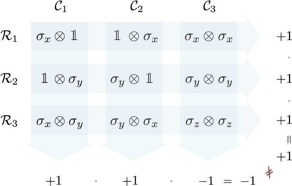
Peres-Mermin Square

Operational Degeneracy from Erasure

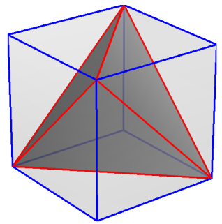
Suppose the corners of the tetrahedron at right are physically distinct states. Any operationally measurable probabilistic mixture uniquely corresponds to a point inside the tetrahedron.

The tetrahedron inscribes a cube, so projecting the tetrahedron to a lower dimension produces a square. The corners of the square still correspond to the original physically distinct states. However, now the interior points can correspond to distinct physical mixtures.

• The tetrahedron is non-contextual: every operationally distinct point inside corresponds to a unique physical mixture.
• The square is contextual: some operationally distinct points can correspond to more than one distinct physical context.
• The latter is obtained from the former by erasing information contained within the projection fibers.

Quantum Contextuality from Erasure?

This erasure model works for finite dimensional probabilistic models.

Can we construct a truly quantum probabilistic space (like the qubit below) in a similar manner from a larger space such that the contextuality in the quantum setting arises explicitly from information erasure?

Spacetime Algebra

Idea : Express known quantum physics (like Dirac electron spin) using algebra, then the erasure that causes contextuality manifests as an algebraic quotient

The physically relevant algebra is the Clifford algebra of spacetime, and contains all relativistic physics (e.g., EM, Dirac theory).

Physical Assumption : Minkowski Metric

• Events can be locally described by a Minkowski pseudo-metric space (+,-,-,-)
   
  • Local velocities (tangent vectors of curves that connect events) must be 4-vectors that obey this metric, according to observed Lorentz symmetries
     
  • Connecting locally flat tangent spaces constructs an event-history manifold
     
• Idea : Construct associative algebra that encodes the metric as a vector contraction
   
  • Yields: (orthogonal) Clifford algebra  \(\text{Cl}_{1,3}(\mathbb{R})\)   ("Spacetime algebra")
    as full geometric tangent space of the event-history manifold
     
    • Nested Subalgebras:    \(\text{Cl}_{1,3}(\mathbb{R}) \supset \text{Cl}_{3,0}(\mathbb{R}) \supset \text{Cl}_{0,2}(\mathbb{R}) \supset \text{Cl}_{0,1}(\mathbb{R}) \supset \mathbb{R} \)
      
                 Bi-Quaternions       \(\text{Cl}_{3,0}(\mathbb{R}) \sim \mathbb{C}\otimes\mathbb{H} \)    (3D space relative to reference frame)
                 Quaternions            \(\text{Cl}_{0,2}(\mathbb{R}) \sim \mathbb{H}\)             (Rotation planes in 3D space)
                 Complex numbers  \(\text{Cl}_{0,1}(\mathbb{R}) \sim \mathbb{C}\)             (Single rotation plane)
                 Real numbers          \(\mathbb{R}\)                                (Measurable quantity)

Constructing Spacetime Algebra

Minkowski Space \(\mathcal{M}_{1,3}(\mathbb{R})\) :

Minkowski metric
(symmetric bilinear form)

Algebraic Axioms:   \(a,b,c\in\mathcal{M}_{1,3}(\mathbb{R})\)

1. Associativity
     \(a(bc) = (ab)c\)
    
2. Left Distributivity
     \(a(b+c) = ab + ac\)
    
3. Right Distributivity
     \((b+c)a = ba + ca\)
    
4. Contraction
     \(a^2 = aa = \eta(a,\,a)\)

Axioms constructively define Clifford algebra \( \text{Cl}_{1,3}(\mathbb{R}) \)

Symmetric part of product encodes metric:

Anti-symmetric part is Grassman wedge product:

(others zero)

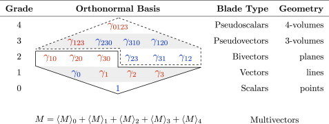
Graded Clifford Basis

• Basis properties:

Grade

0

1

2

3

4

Bivector Planes (of rotation):

3 hyperbolic | 3 elliptic

Vector Lines (of translation):

1 timelike | 3 spacelike

Scalar Points

Pseudovector Volumes:

1 spacelike | 3 timelike

Pseudoscalar 4-Volumes

Multivector:    \( M = \langle M \rangle_0 + \langle M \rangle_1 + \langle M \rangle_2 + \langle M \rangle_3 + \langle M \rangle_4 \)

• Reciprocal basis:

Notational Simplifications

0

1

2

3

(Spacetime-aware "imaginary unit" is the unit pseudoscalar: \(I^2 = -1\))

(commutes with even grade, anti-commutes with odd grade)

4

Relative 3D space embedded as even-graded subspace: \( \text{Cl}_{3,0}(\mathbb{R}) \)

(Observed spatial directions in reference frame)
(Space axis dragged along temporal worldline)

Note duality transformation of left multiplication by \(-I\) : Hodge star operation

Multivector:    \( M = [\alpha + (v_0 + \vec{v})\gamma_0 + \vec{A}] + I[\vec{B} + (w_0 + \vec{w})\gamma_0 + \beta] \)

Quaternions embedded as next even-graded subspace: \( \text{Cl}_{0,2}(\mathbb{R}) \)

Complex numbers embedded as next even-graded subspace: \( \text{Cl}_{0,1}(\mathbb{R}) \)

Connection to Relativistic Formalisms

Proper Form of Multivector:   

\( M = \alpha + v + \mathbf{F} + Iw + I\beta = (\alpha + I\beta) + (v + Iw) + \mathbf{F} \)

Relative Frame Form of Multivector:

\( M = \alpha + (v_0 + \vec{v})\gamma_0 + (\vec{A} + I\vec{B}) + I(w_0 + \vec{w})\gamma_0 + I\beta \)

Tensor Components:

complex scalar

complex vector

bivector

scalar

polar paravector

polar vector

axial vector

axial paravector

pseudoscalar

4-vector

scalar

bivector

pseudovector

pseudoscalar

4-vector components, or a scalar and a relative 3-vector

rank-2 antisymmetric tensor components, or a pair of 3-vectors (one polar, one axial)

Fields and Derivatives

Multivector field:   (in tangent algebra at point \(x\) of spacetime manifold)

\( M(x) = \alpha(x) + v(x) + \mathbf{F}(x) + Iw(x) + I\beta(x) \)

Vector derivative (Dirac operator):

\( \displaystyle \vec{\nabla} \equiv \sum_k \vec{\sigma}^k \frac{\partial}{\partial x^k} \)  ;  \( \vec{\nabla}\vec{v} = \vec{\nabla}\cdot\vec{v} + \vec{\nabla} \wedge \vec{v} = \vec{\nabla}\cdot\vec{v} + (\vec{\nabla}\times \vec{v})I \)    (3-gradient, contains divergence and curl)

\(\nabla^2 = \nabla\gamma_0^2\nabla = (\partial_{ct} - \vec{\nabla})(\partial_{ct} + \vec{\nabla}) = \partial^2_{ct} - \vec{\nabla}\cdot\vec{\nabla} = \Box \)     (d'Alembertian)

Electromagnetism: Maxwell's Equation

electric charge
density and current

This is Maxwell's Equation

Electromagnetic field bivector:

Same form as complex (Riemann-Silberstein) 3-vector

Electromagnetic source complex vector:

magnetic charge
density and current

Contains all of the usual 3D Maxwell's Equations, permitting both electric and magnetic charges

JD, et al. Physics Reports 589 1-71 (2015)

Quantum Particles in Spacetime

To move to quantum mechanics, we must understand the basic quantum objects: the spinors that obey the Dirac equation, and their associated simplifications, the Pauli spinors and Schrodinger wavefunctions

Idempotents, Ideals,
and Quantum Mechanics

• Hilbert space "kets" and "Dirac spinors" in Quantum Mechanics correspond exactly to elements of a left ideal in the spacetime algebra \(\text{Cl}_{1,3}(\mathbb{R})\)
• Hilbert space "bras" and "Dirac adjoint spinors" correspond to associated right ideals
• Hilbert space "operators" correspond to central ideals
• Ideals (right, left, and central) are generated by idempotents in the algebra
• There are three nontrivial classes of idempotents in \(\text{Cl}_{1,3}(\mathbb{R})\):
  
       \( \displaystyle \epsilon_1 = \frac{1 + \gamma_0}{2} \)       \( \displaystyle \epsilon_2 = \frac{1 + \vec{\sigma}_3}{2} \)       \( \displaystyle \epsilon_3 = \frac{1 + \gamma_0 I }{2} \)

Choice of Lorentz Frame

Choice of Spatial Reference within a particular Lorentz Frame

For the simplest case of "nonrelativistic spin", the relevant idempotent is \(\epsilon_2\) 

Hiley, Callaghan, arXiv:1011.4033

  \( \displaystyle \epsilon_1 = \frac{1 + \gamma_0}{2} \)       \( \epsilon_1 = \gamma_0 \, \epsilon_1 \)

Ideals and Dirac Spinors

A left ideal based on \( \epsilon_1 \) reduces the 16-dimensional algebra to an 8-component (Dirac) spinor, equivalent to 4 complex components:
 

The corresponding right ideal is the adjoint spinor:

Their product is the Dirac spinor inner product:

The Dirac spinor can be understood as two quaternions, each equivalent to a Pauli spinor:

\( \Psi \epsilon_1 = [\alpha + \vec{A} + I(\beta + \vec{B})] \epsilon_1  \leftrightarrow \Psi \)

\( \epsilon_1 \tilde{\Psi} = \epsilon_1 [\alpha - \vec{A} + I(\beta - \vec{B})]  \leftrightarrow \bar{\Psi} \)

\( \epsilon_1 \tilde{\Psi}\Psi \epsilon_1 = [|\alpha|^2 - |\vec{A}|^2  - |\beta|^2 + |\vec{B}|^2]\epsilon_1  \leftrightarrow  \bar{\Psi} \Psi \)

\( \Psi \epsilon_1 = [(\alpha + I\vec{B}) + I(\beta - I\vec{A})] \epsilon_1 \\ \qquad = [\psi + I\phi]\epsilon_1  \leftrightarrow \begin{pmatrix}|\psi \rangle \\ |\phi \rangle \end{pmatrix} \)

\( \epsilon_1 \tilde{\Psi}\Psi \epsilon_1 \leftrightarrow  \langle \psi | \psi \rangle - \langle \phi | \phi \rangle \)

  \( \displaystyle \epsilon_2  = \frac{1 + \vec{\sigma}_3}{2} \)       \( \epsilon_2 = \vec{\sigma}_3 \, \epsilon_2 \)         \( \displaystyle \epsilon_1 = \frac{(1-\gamma_3)\epsilon_2(1 + \gamma_3)}{2} = \frac{(1 + \gamma_0)\epsilon_2(1 + \gamma_0)}{2}\)

Ideals and Pauli Spinors

An equivalent left ideal based on \( \epsilon_2 \) directly isolates the relevant Pauli spinors:

\( \Psi \epsilon_2 = [(\alpha + I\vec{B}) + (v_0 + I\vec{w})\gamma_0] \epsilon_2  = [\psi + \phi\gamma_0]\epsilon_2 \)

\( \psi\epsilon_2 = [\alpha + I\vec{B}]\epsilon_2 = [(\alpha + B_3 I) + (B_2 - B_1 I) I\vec{\sigma}_2] \epsilon_2 \)

\(\epsilon_2 \leftrightarrow |0\rangle \)

\( I\vec{\sigma}_2\epsilon_2 \leftrightarrow i\hat{\sigma}_2|0\rangle = |1\rangle \)

\( \psi\epsilon_2 = (\alpha + I\vec{B})\epsilon_2 \leftrightarrow (\alpha + B_3 I)|0\rangle + (B_2 - B_1 I)|1\rangle = |\psi\rangle \)

For nonrelativistic cases, the first Pauli spinor is sufficient, and produces a spin qubit:

Left ideal \(\leftrightarrow\) Pauli Spinors/Kets

Central ideal \(\leftrightarrow\) Operators

\(\epsilon_2 \leftrightarrow |0\rangle\langle 0 | \)

\( (I\vec{\sigma}_2)\epsilon_2(-I\vec{\sigma}_2) \leftrightarrow |1\rangle\langle 1 | \)

\( \psi\epsilon_2\tilde{\psi} \leftrightarrow |\psi \rangle\langle \psi | \)

Reduction as Erasure

• The progression from the full algebra \(\text{Cl}_{1,3}(\mathbb{R})\) to a qubit can be understood as a succession of projections that erase information:
  • Selecting an ideal isolates a Dirac spinor:
    \( M \in \text{Cl}_{1,3}(\mathbb{R}) \mapsto M\epsilon_2 = \Psi\epsilon_2 \),   \(\Psi \in \text{Cl}_{3,0} \sim \mathbb{C}\otimes\mathbb{H} \)
  • Eliminating boosts isolates a Pauli spinor:
    \(\Psi\epsilon_2 \mapsto \langle\Psi\epsilon_2\rangle_{\text{even}} = \psi\,\epsilon_2 \),    \(\psi \in \text{Cl}_{0,2} \sim \mathbb{H}\)
  • Keeping only one spatial axis isolates a Schrodinger wavefunction:
    \(\psi\,\epsilon_2 \mapsto \epsilon_2\psi\epsilon_2 = \psi_z\,\epsilon_2 \),    \(\psi_z \in \text{Cl}_{0,1} \sim \mathbb{C} \)
• This nesting of algebras exactly mirrors the even-graded subalgebras:
      \( \text{Cl}_{1,3}(\mathbb{R}) \supset \text{Cl}_{3,0}(\mathbb{R}) \supset \text{Cl}_{0,2}(\mathbb{R}) \supset \text{Cl}_{0,1}(\mathbb{R}) \)
      Multivector \(\supset\) Dirac spinor \(\supset\) Pauli spinor \(\supset\) Schrodinger Wavefunction
   
• In this precise sense, one must erase information from a larger geometric space to obtain the relevant quantum space

Multi-particle Erasure

• This erasure becomes even more striking with two particles :
  • To obtain a "tensor product" within the algebra that behaves correctly, one has to duplicate the entire spacetime: \( \text{Cl}(\mathcal{M}_{1,3}\oplus\mathcal{M}_{1,3}) \)
  • This creates a dimensionality of \(2^{4+4} = 256\), which is far too large (should be 8)
  • The correct quantum space of two nonrelativistic spins is obtained after not just projecting to separate ideals on each spacetime, but by projecting onto an ideal of a correlated idempotent that glues together reference orientations of the independent spacetimes
             
               \( \displaystyle \epsilon_{22} = \frac{1 + \vec{\sigma}^{(1)}_3\vec{\sigma}^{(2)}_3}{2}  \leftrightarrow |0\rangle|0\rangle \),                   \( \displaystyle \exp(-I \sum_{ij}h_{ij}\vec{\sigma}^{(1)}_i\vec{\sigma}^{(2)}_j)\,\epsilon_{22} \leftrightarrow |\Psi\rangle \)
     
  • This gluing procedure permits entanglement between the particles: the most well-known consequence of contextuality!
    
             \( \displaystyle \frac{1 - \vec{\sigma}^{(1)}_1\vec{\sigma}^{(2)}_1}{\sqrt{2}}\frac{1 - \vec{\sigma}^{(1)}_3\vec{\sigma}^{(2)}_3}{2} \leftrightarrow \frac{|1\rangle|0\rangle - |0\rangle|1\rangle}{\sqrt{2}} \)

Notably an entangled state can be understood directly as a product of correlated idempotents that identify spin axes of both particles 

Conclusions 

• Spacetime Clifford algebra is the natural language of relativistic physics
   
• Multiparticle quantum mechanics is constructed algebraically as a correlated ideal within redundant copies of spacetime
   
• There is a close correspondence between the erasure of information inherent to the procedure of forming ideals and the operational degeneracy that appears in the form of quantum contextuality

Thank you!