Introduction:
Hydrogen in fusion
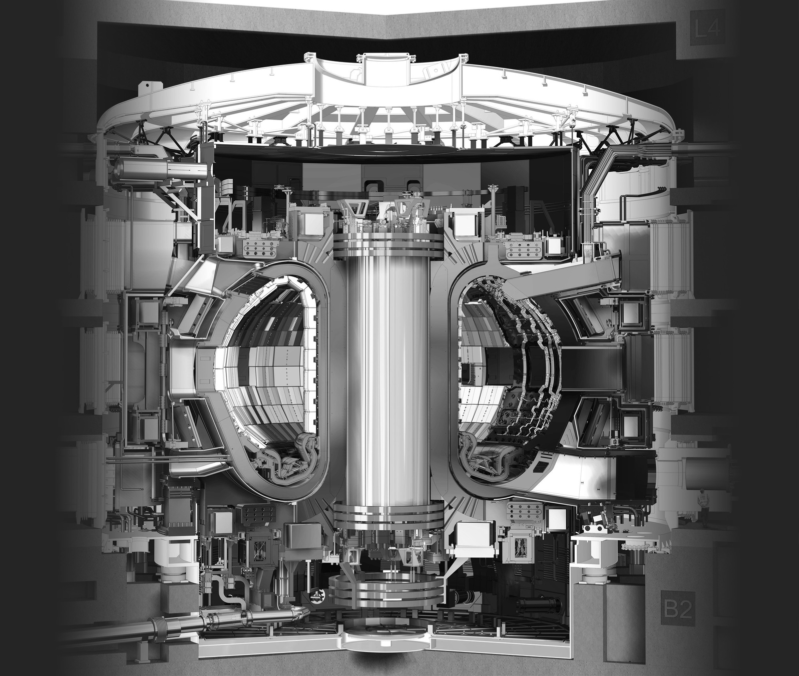
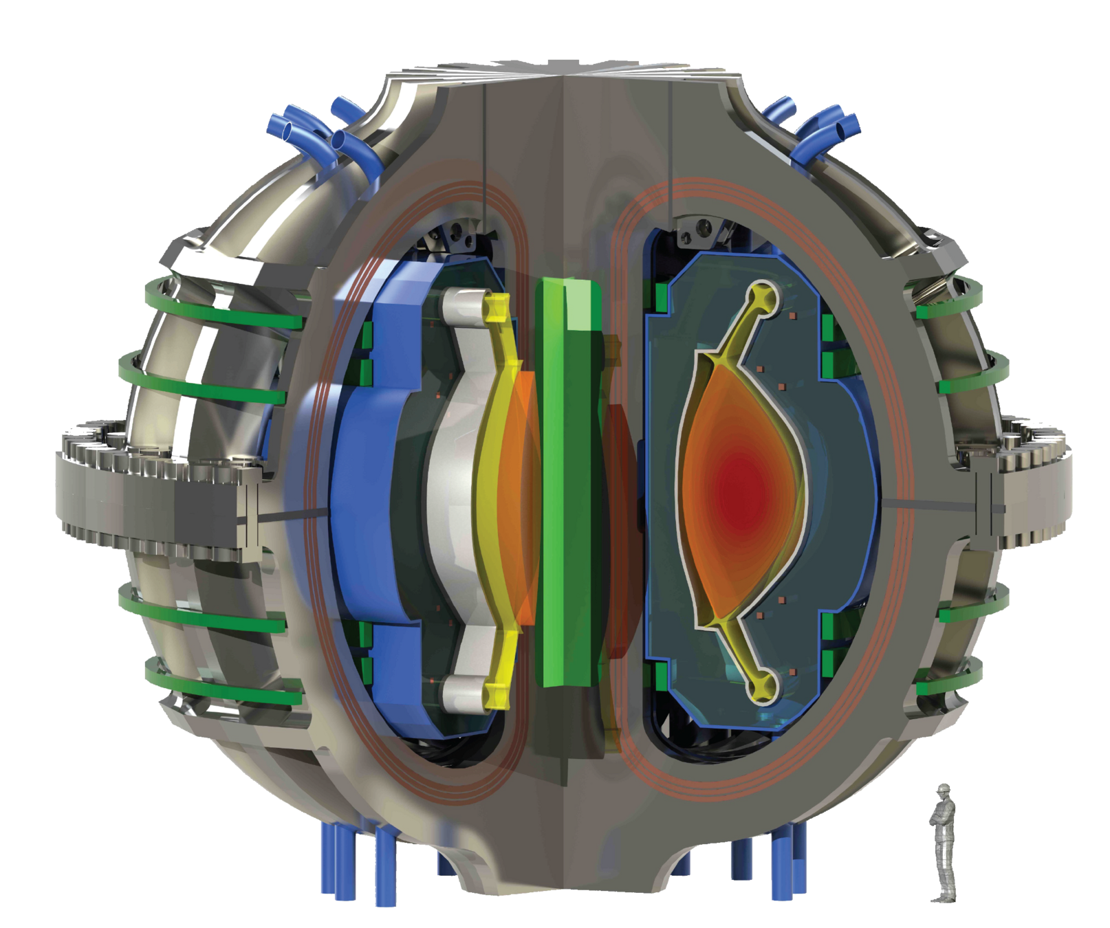
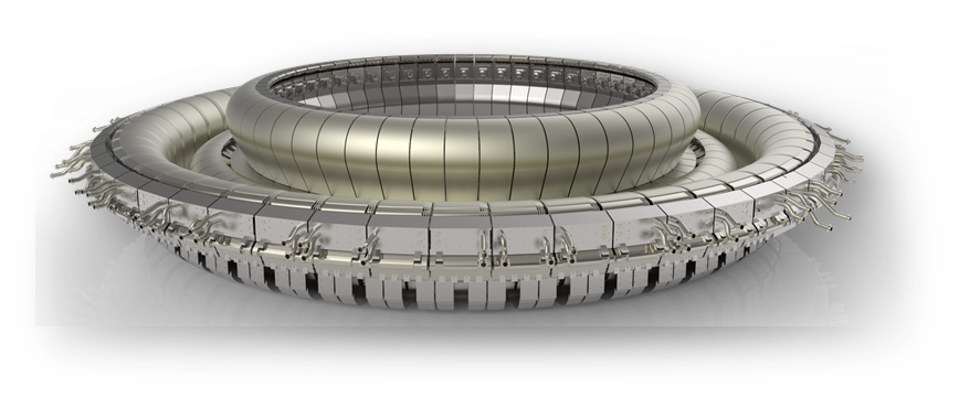
ITER
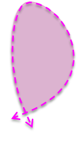
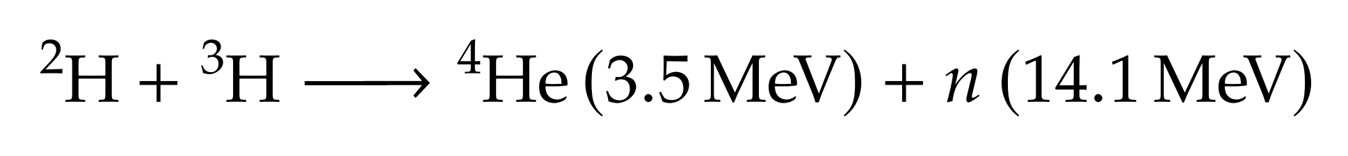
Plasma: mixture of Hydrogen (D-T) and Helium
Particle bombardment
Divertor
Why should we care?
T is rare
T is expensive
€£$
Material embrittlement
T is radioactive
☢
What's Tritium?
+
+
+
Protium
Deuterium
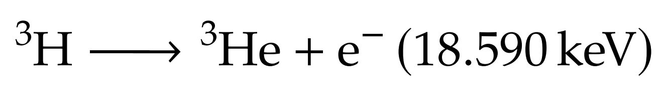
Tritium
Molar mass: 6.032 g/mol
What's Tritium?
+
Tritium
☢
800 \ \text{MWth} \approx 10^{20} \ \text{reactions/s} \approx 100 \ \text{kg/year}
Consumption in a single fusion reactor:
What's Tritium?
+
Tritium
☢
Half-life: 12 years
☢
World production:
- CANDU reactors (Canadian Deuterium Uranium): 130 g per year
- From cosmic rays: 200 g per year
We need to produce tritium!
World reserves:
\( \approx \) 100 kg
Cost: $30,000 per gram
Fuel self-sufficiency
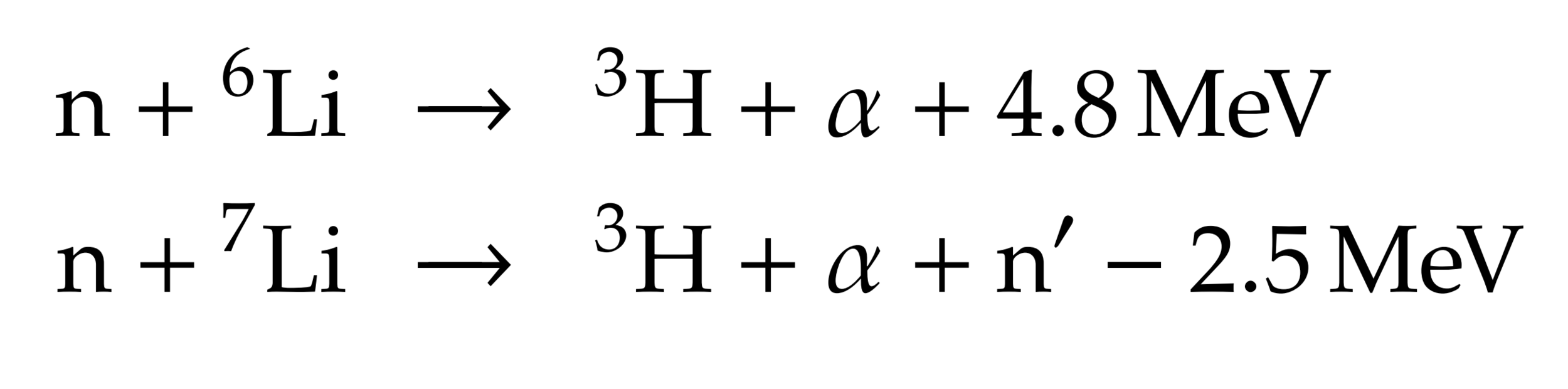
Lithium is used to breed tritium
\mathrm{TBR} = \mathrm{\frac{tritium \ produced}{tritium \ consumed}}
🎯Goals
↗️Maximise TBR
↘️Minimise volume
Lithium is used to breed tritium
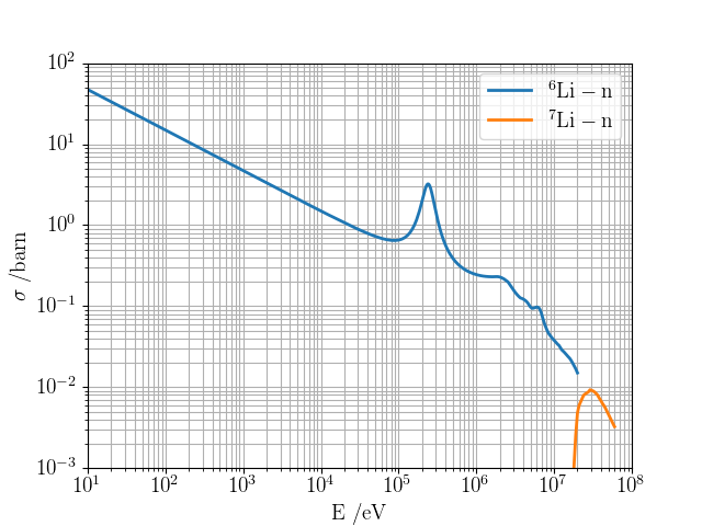
→ Li6 enrichment is an option
DT fusion neutrons

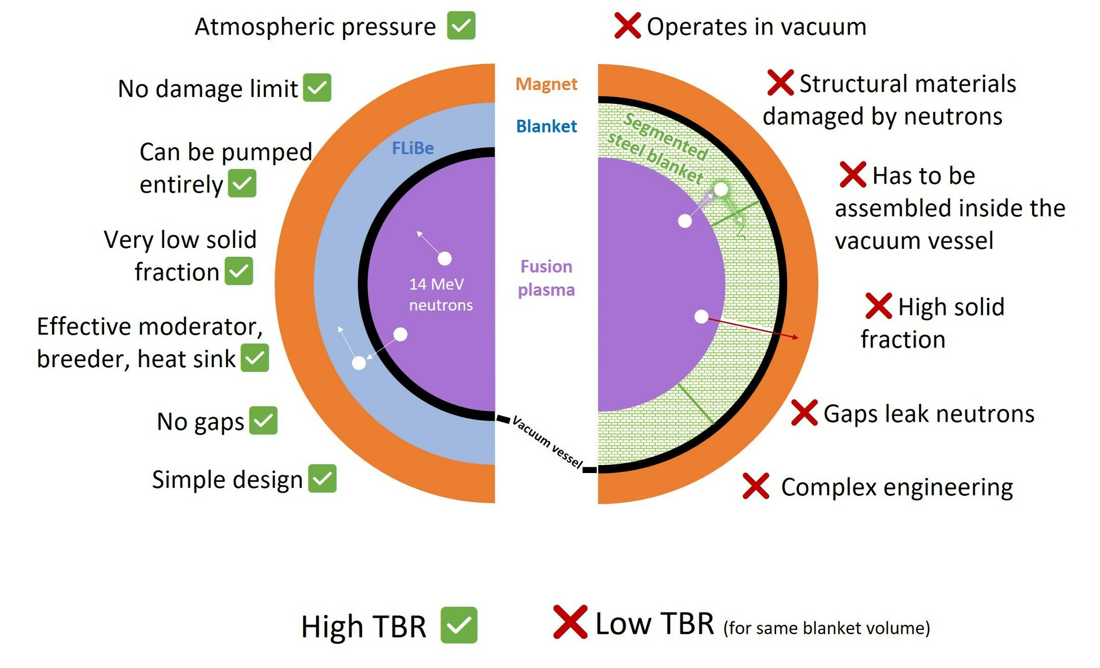
There are several concepts of breeding blanket
FLiBe
Li
LiPb
Choose your breeder
Li in ceramics
There are several concepts of breeding blanket
FLiBe
Li
LiPb
Self
Water
He
He+Water
Choose your breeder
Choose your coolant
Li in ceramics
There are several concepts of breeding blanket
FLiBe
Li
LiPb
Self
Water
He
He+Water
Liquid
Segmented
Choose your breeder
Choose your coolant
Choose your geometry
Li in ceramics
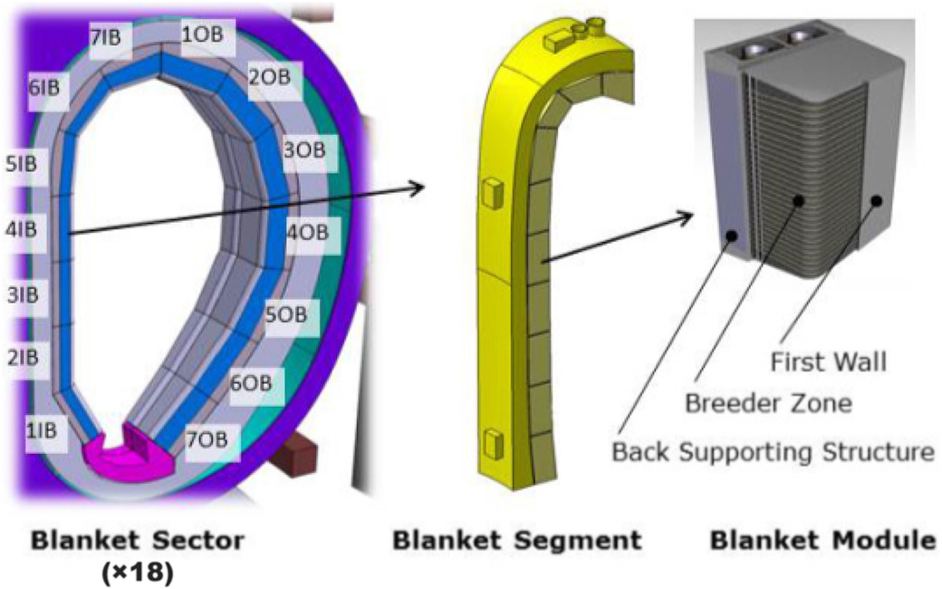
Froio et al Fus Eng Design 2017
There are several concepts of breeding blanket
FLiBe
Li
LiPb
Self
Water
He
He+Water
Liquid
Segmented
Choose your breeder
Choose your coolant
Choose your geometry
Li in ceramics
ARC's liquid immersion blanket
There are several concepts of breeding blanket
FLiBe
Li
LiPb
Self
Water
He
He+Water
Liquid
Segmented
Choose your breeder
Choose your coolant
Choose your geometry
Li in ceramics
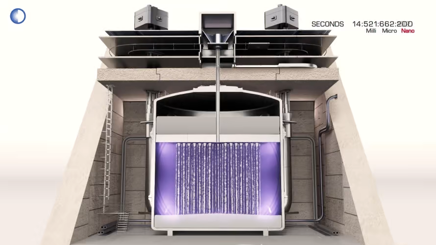
First Light Fusion
There are several concepts of breeding blanket
FLiBe
Li
LiPb
Self
Water
He
He+Water
Liquid
Segmented
Choose your breeder
Choose your coolant
Choose your geometry
Li in ceramics
Water Cooled Lithium-Lead
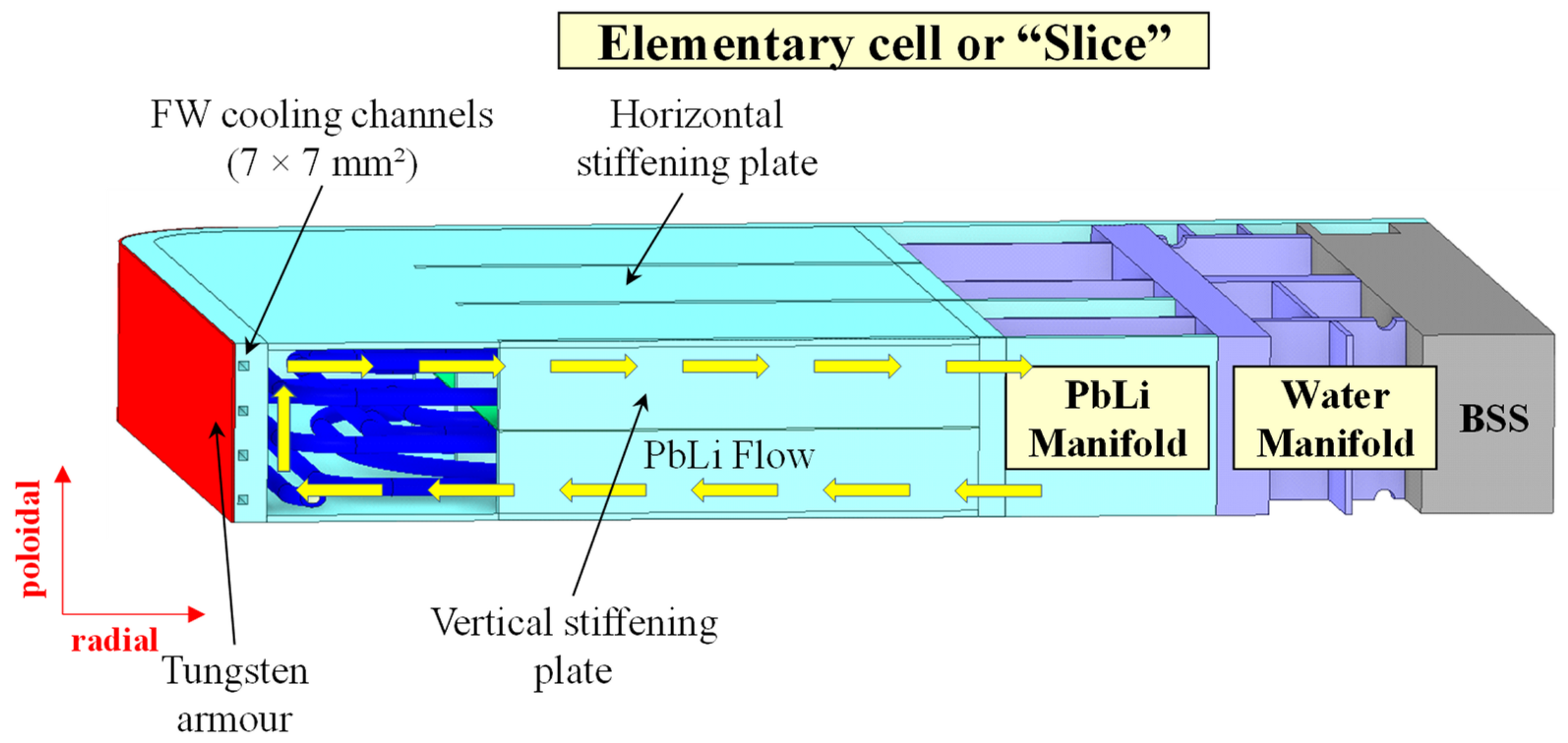
Arena et al Energies 2023, 16, 2069
Segmented vs LIB
The breeding blanket is only one component of the fuel cycle
- Need to understand how tritium behaves in each of these components
- cf. Fuel Cycle Modelling
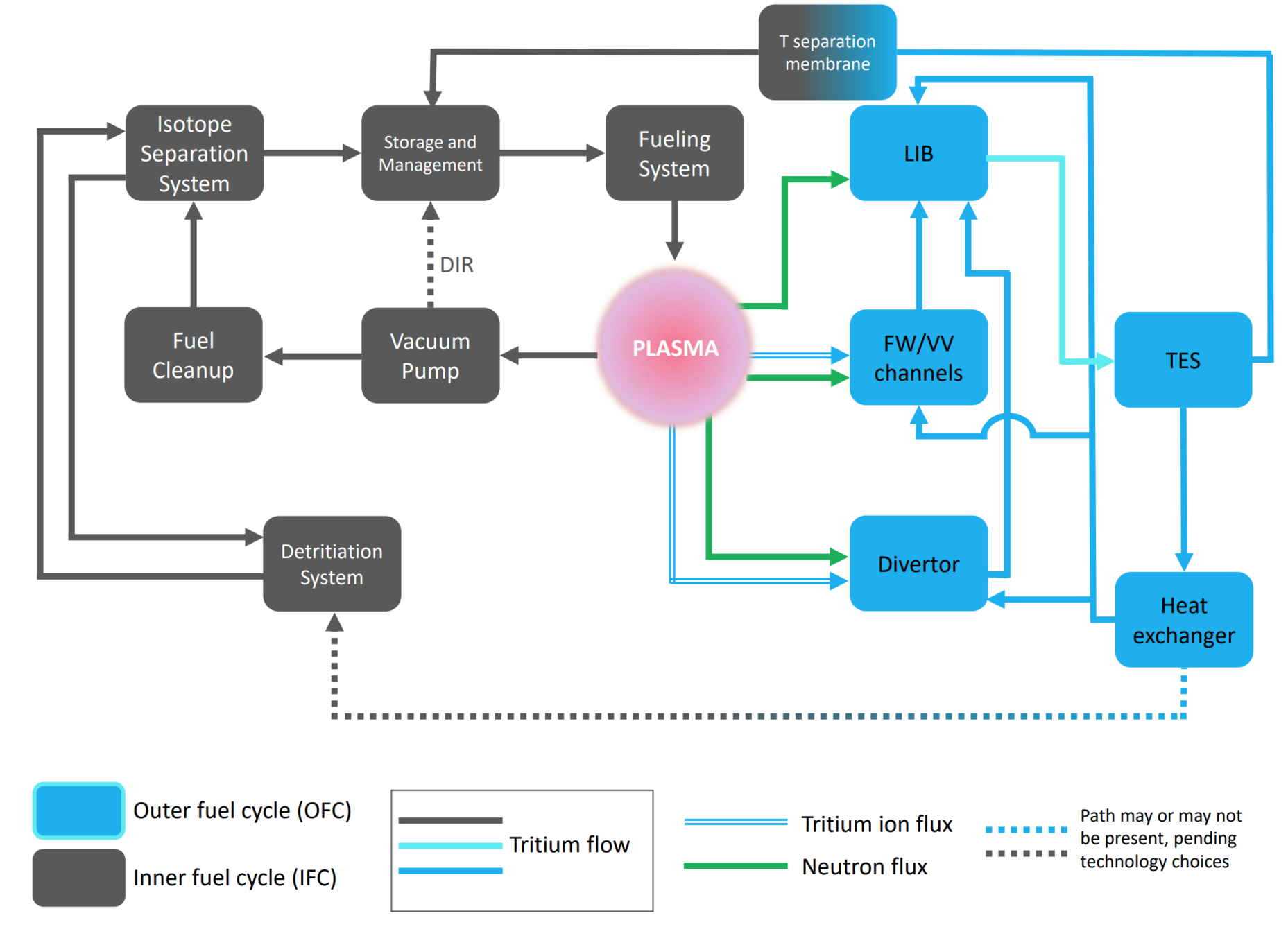
Meschini et al (submitted)
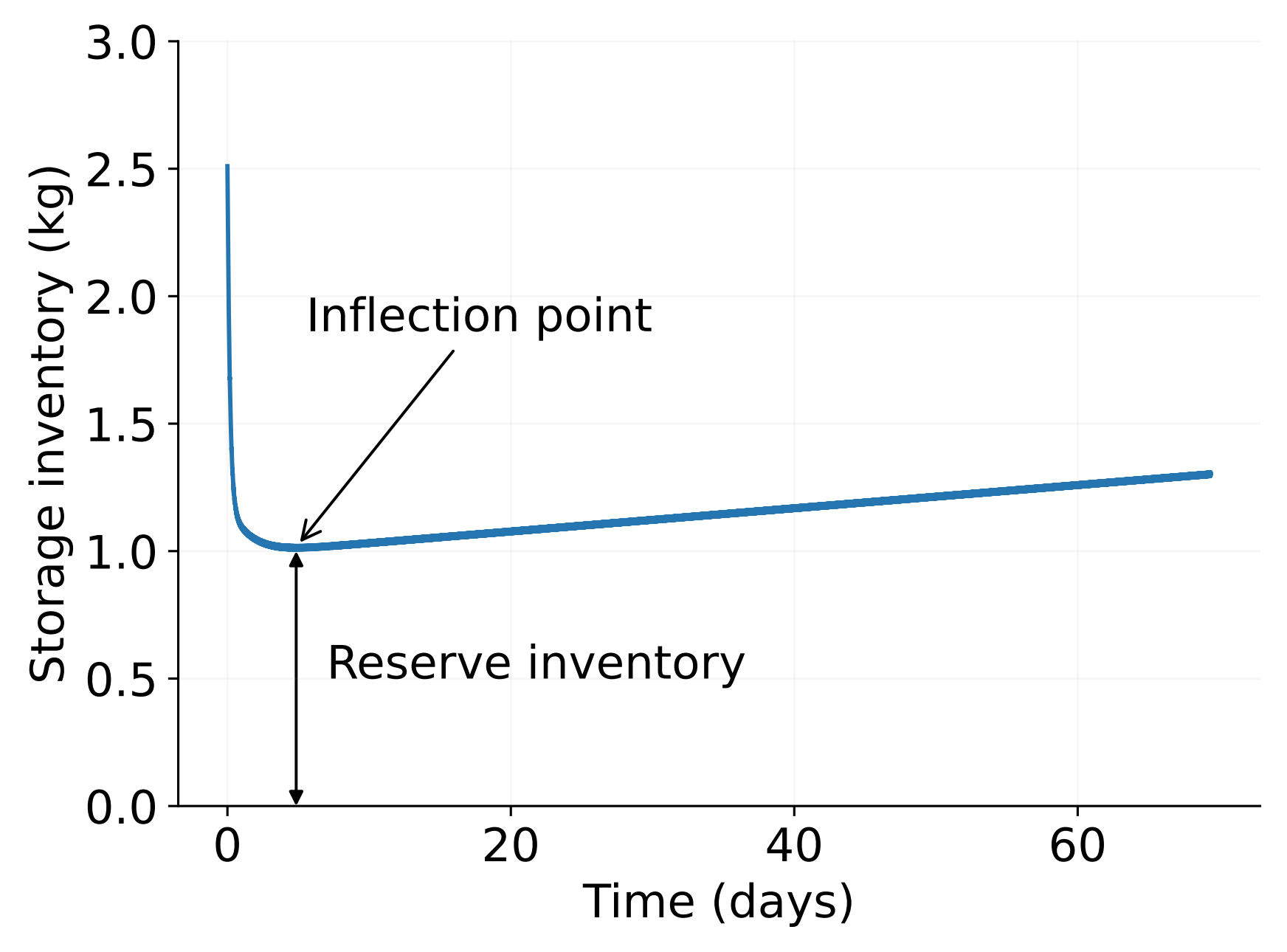
A startup inventory of T is required
Meschini et al (submitted)
The efficiency of the fuel cycle will influence the future fusion economy
- Doubling time: time required for a reactor to produce enough tritium to start another reactor
- Energy industry: \(\tau_2 \approx \) 2-3 years
- Constrains the required TBR and the startup inventory
- Different fuel cycles can give different TBRr and startup inventories
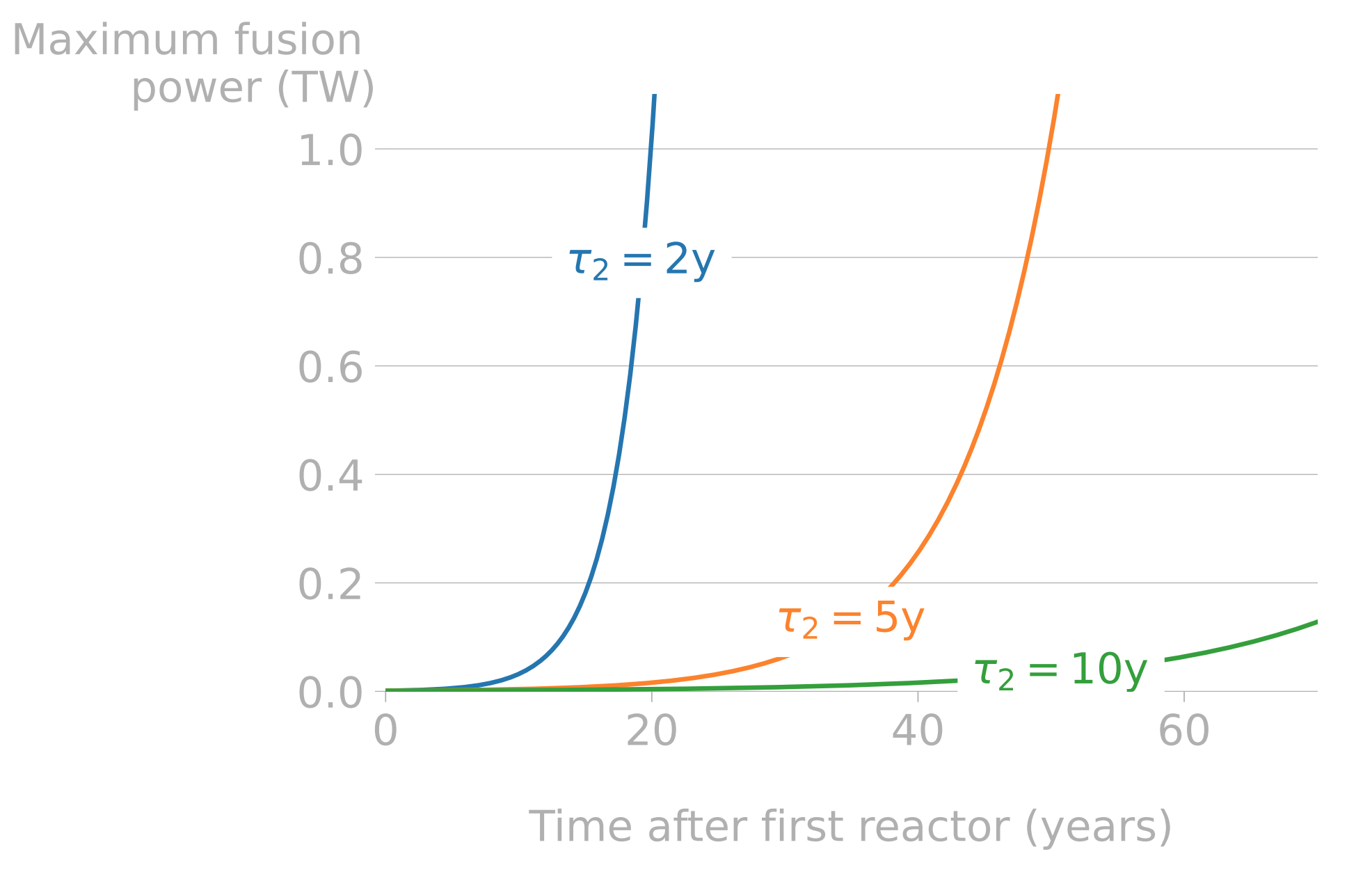
P_\mathrm{max} = P_\mathrm{plant} \times 2^{t/\tau_2}
Safety
Tritium is a health hazard
☢
- No external hazard: electron stopped by skin
- Once ingested, can cause damage to internal tissues
- Forms: HT, HTO, methane, titrides...
- Biological half-life of HTO: 10 days
- Biological half-life of OBT (Organically Bound Tritium): 40 days
Augustin Janssens. ‘Emerging Issues on Tritium and Low Energy Beta Emitters”’. en. In: (Nov. 2007), p. 100
| Country | Water limit (Bq/L) |
|---|---|
| EU | 100 |
| USA | 740 |
| UK | 100 |
| Canada | 7,000 |
| Finland | 30,000 |
| Australia | 76,103 |
| Russia | 7,700 |
| WHO | 10,000 |
The content of tritium needs to be limited
1. Keep inventory at a minimum
Tritium limit in the ITER vacuum vessel: 1 kg
The content of tritium needs to be limited
1. Keep inventory at a minimum
2. Reduce inventory
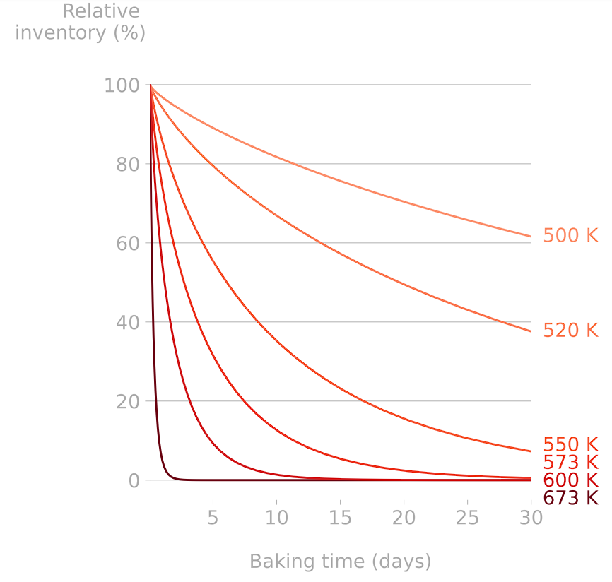
Heating components help releasing their tritium content (cf. Basics of H transport)
The content of tritium needs to be limited
1. Keep inventory at a minimum
2. Reduce inventory
3. Avoid contamination of coolants
Metal
Tritiated environment
"Clean" environment
Permeation
The content of tritium needs to be limited
1. Keep inventory at a minimum
2. Reduce inventory
3. Avoid contamination of coolants
Metal
Tritiated environment
"Clean" environment
Permeation
Permeation barrier
The content of tritium needs to be limited
1. Keep inventory at a minimum
2. Reduce inventory
3. Avoid contamination of coolants
Ceramics are promising candidates:
- oxides
- carbides
- nitrides
Permeation barriers are caracterised by their PRF (Permeation Reduction Factor)
\mathrm{PRF} = \frac{\mathrm{uncoated \ flux}}{\mathrm{coated \ flux}}
Target for breeding blankets PRF ≈ 100-1000
Luo et al Surface and Coatings Technology 2020
Component embrittlement
Agglomeration of hydrogen can lead to blistering
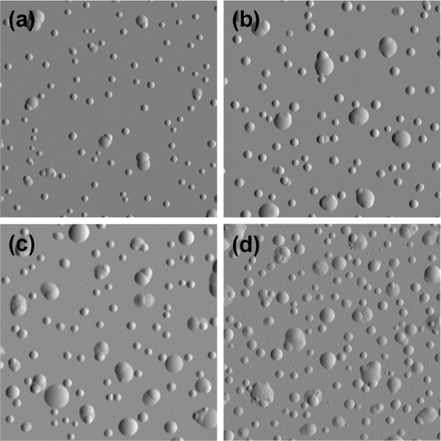
- Accumulation of H at defects:
- Voids
- Reaction with impurities (formation of methane)
- grain boundaries
- Creation of a filled cavity
- Growth of the cavity without bursting
Kuznetsov, Alexey S. et al. “Hydrogen-induced blistering of Mo/Si multilayers: Uptake and distribution.” Thin Solid Films 545 (2013): 571-579.
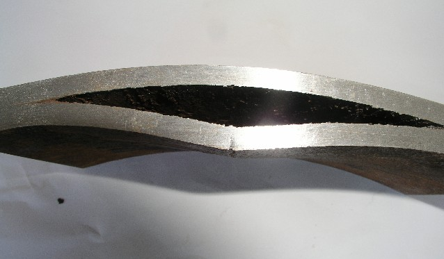
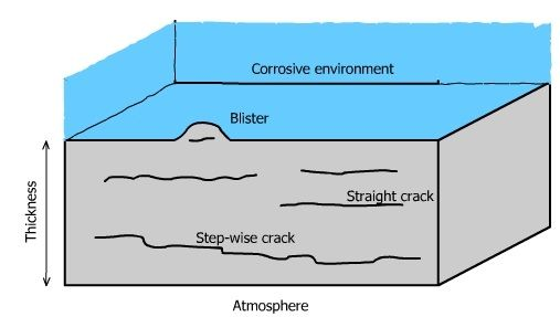
Cavities can lead to Hydrogen Induced Cracking
Review of HIC by Sofronis
https://doi.org/10.1016/j.jngse.2022.104547
Take aways
H transport
Safety
Fusion Economy
Materials
- Minimising inventories
- Limiting permeation
- Protecting personel
- Fuel cycle
- Tritium breeding
- Losses
- Embrittlement
- H induced cracks
Question time!
Fundamentals of hydrogen transport in materials
Outline
- Sources of H transport in fusion (2 mins)
- Basics of H transport (10 mins)
- Surface effects (Sievert vs Henry, recombination, dissociation,)
- Bulk diffusion (Fick, Soret...)
- Interfaces
- Trapping (intrinsic, extrinsic)
- Isotopic exchange
What are the sources of tritium in a tokamak?
1. Direct implantation from the plasma
2. Neutron capture from Lithium
3. Neutron capture by Helium-3
Hydrogen transport in metals
Diffusion
Even more particles:
continuity approximation
1 particle:
Random walk
Many particles
Diffusion
\varphi_\mathrm{diffusion} = - D \ \nabla c
\( \varphi_\mathrm{diffusion} \): diffusion flux
\( D \): diffusion coefficient
\( c \): diffusive hydrogen concentration
Fick's first law of diffusion
Diffusion
\varphi_\mathrm{diffusion} = - D \ \nabla c
\( \varphi_\mathrm{diffusion} \): diffusion flux
\( D \): diffusion coefficient
\( c \): diffusive hydrogen concentration
\( S\): source term
Fick's 1st law of diffusion
\frac{\partial c}{\partial t} = - \nabla \cdot \varphi_\mathrm{diffusion} + S
Fick's 2nd law of diffusion
Diffusion
\varphi_\mathrm{diffusion} = - D \ \left( \nabla c + \frac{Q\ c}{R \ T^2} \ \nabla{T} - \frac{c \ V_H}{R \ T} \nabla \sigma \right)
\( \varphi_\mathrm{diffusion} \): diffusion flux
\( D \): diffusion coefficient
\( c \): diffusive hydrogen concentration
\( S\): source term
Soret effect (or thermophoresis)
Stress assisted diffusion
Particle implantation
Ziegler et al. 2010. Nuclear Instruments and Methods in Physics Research Section B: Beam Interactions with Materials and Atoms, 268 (11): 1818–23. https://doi.org/10.1016/j.nimb.2010.02.091.
Implantation range
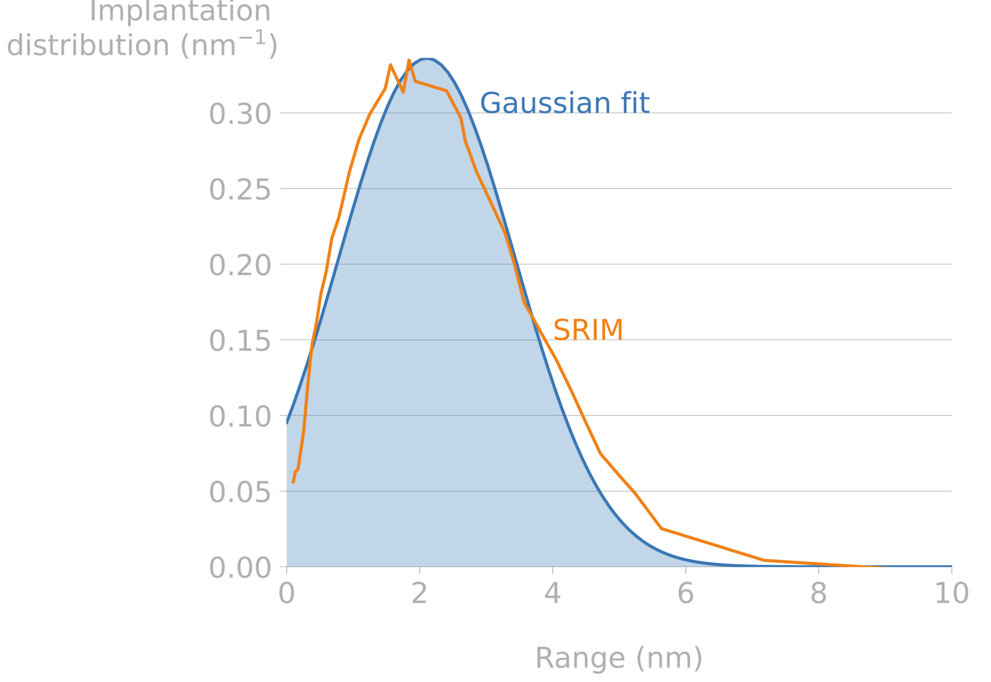
Implantation range & width and reflection coefficient can be computed with SRIM, SDTRIM...
Mutzke et al, SDTrimSP Version 6.00 2019
Particle implantation
S = (1-r) \ \Gamma_\mathrm{incident} \ f(x)
\(\Gamma_\mathrm{incident} \): incident flux (particle/m2/s)
\( f(x) \): Gaussian distribution (/m)
\(r \): reflection coefficient
Transport in liquids
Advection + diffusion
Carrying H in the liquid flow
Normal diffusion process
Requires to do some Computational Fluid Dynamics
Transport in liquids
Advection + diffusion
Carrying H in the liquid flow
Normal diffusion process
Requires to do some Computational Fluid Dynamics
Correlations
Transport in liquids
Heat transfer analogy
H transport
q = h \ (T_\infty - T_0)
\varphi = k \ (c_\infty - c_0)
\(T_\infty\)
\(T_0\)
\(c_\infty\)
\(c_0\)
Transport in liquids
Heat transfer analogy
H transport
q = h \ (T_\infty - T_0)
\varphi = k \ (c_\infty - c_0)
\( h \): heat transfer coefficient (W/K/m2)
\( k \): mass transport coefficient (m/s)
Nu = a\ Re^b \ Pr^c
Sh = a\ Re^b \ Sc^c
Nu = \frac{h}{\lambda/L} = \frac{\mathrm{Convective \ rate}}{\mathrm{Conduction \ rate}}
Sh = \frac{k}{D/L} = \frac{\mathrm{Convective \ rate}}{\mathrm{Diffusion \ rate}}
Surface effects
H2 molecules
Metal lattice
Surface effects
\varphi_\mathrm{dissociation} = K_\mathrm{d} \ P
Dissociation coefficient (H/m2/s/Pa)
Partial pressure of H (Pa)
Adsorbed H
Metal lattice
Surface effects
\varphi_\mathrm{dissociation} = K_\mathrm{d} \ P
\varphi_\mathrm{recombination} = K_\mathrm{r} \ c^2
Metal lattice
Recombination coefficient (m4/s)
Concentration (H/m3)
Surface effects
\varphi_\mathrm{dissociation} = K_\mathrm{d} \ P
\varphi_\mathrm{recombination} = K_\mathrm{r} \ c^2
Metal lattice
\varphi_\mathrm{net} = \varphi_\mathrm{dissociation} - \varphi_\mathrm{recombination}
Waelbroeck model
Surface effects
\varphi_\mathrm{dissociation} = K_\mathrm{d} \ P
\varphi_\mathrm{recombination} = K_\mathrm{r} \ c^2
Metal lattice
At equilibrium:
\varphi_\mathrm{net} = 0
c = \sqrt{\frac{K_\mathrm{d}}{K_\mathrm{r}}} \ \sqrt{P}
\varphi_\mathrm{net} = \varphi_\mathrm{dissociation} - \varphi_\mathrm{recombination}
c = S \ \sqrt{P}
Sievert's law of solubility
Surface effects
\varphi_\mathrm{dissociation} = K_\mathrm{d} \ P
\varphi_\mathrm{recombination} = K_\mathrm{r} \ c^\textcolor{black}{1}
Non-metallic liquid
At equilibrium:
\varphi_\mathrm{net} = 0
c = \textcolor{black}{\frac{K_\mathrm{d}}{K_\mathrm{r}} \ P}
\varphi_\mathrm{net} = \varphi_\mathrm{dissociation} - \varphi_\mathrm{recombination}
c = K_H \ P
Henry's law of solubility
Interfaces
Material 1
Material 2
Interfaces
Partial pressure and flux are continuous
Material 1
Material 2
Interfaces
Material 1
Material 2
Case 1:
Metal-Metal
- D_1 \nabla c_1 = - D_2 \nabla c_2
P = \left( \frac{c}{K_S} \right) ^2
\left( \frac{c_1}{K_{S,1}} \right)^2 =\left( \frac{c_2}{K_{S,2}} \right)^2
Sievert's law
Interfaces
Material 1
Material 2
Case 2:
Non metal-non metal
- D_1 \nabla c_1 = - D_2 \nabla c_2
P = \frac{c}{K_H}
\frac{c_1}{K_{H,1}} = \frac{c_2}{K_{H,2}}
Henry's law
Interfaces
Material 1
Material 2
Case 3:
Metal-Non metal
- D_1 \nabla c_1 = - D_2 \nabla c_2
P = \left( \frac{c}{K_S} \right) ^2
\left( \frac{c_1}{K_{S,1}} \right)^2 = \frac{c_2}{K_{H,2}}
Sievert's law
P = \frac{c}{K_H}
Henry's law
Interfaces
Material 1
Material 2
Steady state concentration profile
- different diffusivities \(\rightarrow\) different concentration gradients
- different solubilities \( \rightarrow \) concentration discontinuity
\(x\)
\(c\)
Permeation barriers are low solubility, low duffisivity
Metal
Tritiated environment
"Clean" environment
Permeation
Permeation barrier
Permeation barriers are low solubility, low duffisivity
Pressure \(P\)
High gradient = high flux
Low gradient = low flux
c
c
Pressure \(P\)
Trapping
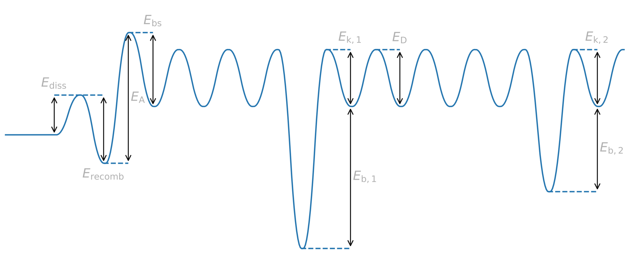
H
Trap = anything binding to H
- vacancy
- grain boundary
- impurity
- chemical reaction
- ...
Trapping
H
Potential energy
Distance
Diffusion barrier
Energy barrier = activation energy
Trap binding energy
Trapping energy
Common assumption:
\( E_k = E_D \)
Trapping
\mathrm{H} + [\ \ \ ]_\mathrm{trap} \ \substack{p \\[-1em] \longleftarrow\\[-1em] \longrightarrow \\[-1em] k} \ [\mathrm{H}]_\mathrm{trap}
0D
\frac{\partial c_\mathrm{t}}{\partial t} = -\frac{\partial c_\mathrm{m}}{\partial t} = k \ c_\mathrm{m} \ n_\mathrm{free \ trap} - p c_\mathrm{t}
c_\mathrm{t}
Since \(n_\mathrm{trap} = n_\mathrm{free \ trap} + c_\mathrm{t} \)
c_\mathrm{m}
n_\mathrm{free \ trap}
Trapping
\mathrm{H} + [\ \ \ ]_\mathrm{trap} \ \substack{p \\[-1em] \longleftarrow\\[-1em] \longrightarrow \\[-1em] k} \ [\mathrm{H}]_\mathrm{trap}
0D
\frac{\partial c_\mathrm{t}}{\partial t} = -\frac{\partial c_\mathrm{m}}{\partial t} = k \ c_\mathrm{m} \ (n_\mathrm{trap,0} - c_\mathrm{t}) - p c_\mathrm{t}
c_\mathrm{m}
n_\mathrm{free \ trap}
c_\mathrm{t}
Total concentration of traps
Trapping
0D
\frac{\partial c_\mathrm{t}}{\partial t} = -\frac{\partial c_\mathrm{m}}{\partial t} = k \ c_\mathrm{m} \ (n_\mathrm{trap,0} - c_\mathrm{t}) - p c_\mathrm{t}
With diffusion
and
1 trap
\frac{\partial c_\mathrm{m}}{\partial t} = \nabla \cdot \left(D\nabla c_\mathrm{m} \right) + S - \frac{\partial c_\mathrm{t}}{\partial t}
\frac{\partial c_\mathrm{t}}{\partial t} = k \ c_\mathrm{m} \ (n_\mathrm{trap,0} - c_\mathrm{t}) - p c_\mathrm{t}
Trapping
3 traps
\frac{\partial c_\mathrm{m}}{\partial t} = \nabla \cdot \left(D\nabla c_\mathrm{m} \right) + S - \sum \frac{\partial c_\mathrm{t,i}}{\partial t}
\frac{\partial c_\mathrm{t, 1}}{\partial t} = k_1 \ c_\mathrm{m} \ (n_\mathrm{trap,1} - c_\mathrm{t,1}) - p_1 c_\mathrm{t,1}
\frac{\partial c_\mathrm{t, 2}}{\partial t} = k_2 \ c_\mathrm{m} \ (n_\mathrm{trap,2} - c_\mathrm{t,2}) - p_2 c_\mathrm{t,2}
\frac{\partial c_\mathrm{t, 3}}{\partial t} = k_3 \ c_\mathrm{m} \ (n_\mathrm{trap,3} - c_\mathrm{t,3}) - p_3 c_\mathrm{t,3}
McNabb & Foster model
Trapping
Other models assume traps can hold more than one H
\mathrm{H} + [\ \ \ ]_\mathrm{trap} \ \substack{p_1 \\[-1em] \longleftarrow\\[-1em] \longrightarrow \\[-1em] k_1} \ [\mathrm{H}_1]_\mathrm{trap}
\mathrm{H} + [\mathrm{H}_1]_\mathrm{trap} \ \substack{p_2 \\[-1em] \longleftarrow\\[-1em] \longrightarrow \\[-1em] k_2} \ [\mathrm{H}_2]_\mathrm{trap}
\mathrm{H} + [\mathrm{H}_2]_\mathrm{trap} \ \substack{p_3 \\[-1em] \longleftarrow\\[-1em] \longrightarrow \\[-1em] k_3} \ [\mathrm{H}_3]_\mathrm{trap}
\frac{\partial c_\mathrm{m}}{\partial t} = \nabla \cdot \left(D\nabla c_\mathrm{m} \right) + S - \sum{k_{i} \ c_\mathrm{m} \ c_{\mathrm{t},i-1} - p_i c_{\mathrm{t},i}}
\frac{\partial c_{\mathrm{t},i}}{\partial t} = k_{i} \ c_\mathrm{m} \ c_{\mathrm{t},i-1} - p_i c_{\mathrm{t},i} - k_{i+1} \ c_\mathrm{m} \ c_{\mathrm{t},i} + p_{i+1} c_{\mathrm{t},i+1}
Many of these processes are thermally activated
Recombination
Dissociation
Absorption
Trapping
Detrapping
Diffusion
Arrhenius law
X = X_0 \ \exp{\left(\frac{-E_X}{k_B \ T}\right)}
Pre-exponential factor
Activation energy (eV/H)
Temperature (K)
Boltzmann constant (eV/H/K)
k_B = 8.617\times 10^{-5} \ \mathrm{eV/H/K}
Arrhenius law
X = X_0 \ \exp{\left(\frac{-E_X}{R \ T}\right)}
Pre-exponential factor
Activation energy (J/mol)
Temperature (K)
Gas constant (J/mol/K)
k_B = 8.617\times 10^{-5} \ \mathrm{eV/H/K}
R = 8.314 \ \mathrm{eV/H/K}
\frac{E_D [eV/H]}{k_B} = \frac{E_D [J/mol]}{R}
Conversion:
Arrhenius law
X = X_0 \ \exp{\left(\frac{-E_X}{R \ T}\right)}
\( 1/T \) (1/K)
E_X > 0
E_X < 0
Arrhenius law
X = X_0 \ \exp{\left(\frac{-E_X}{R \ T}\right)}
\log{(X)} = \log{(X_0)} \ - \frac{E_X}{k_B \ T}
\log{(X)} = \log{(X_0)} \ - \frac{E_X}{k_B} \ \frac{1}{T}
Intercept
+ Slope
Y =
X
Arrhenius law
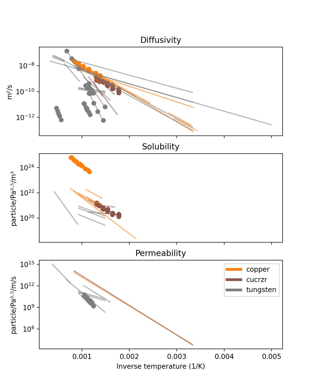
Arrhenius parameters:
- Diffusivity
- Solubility
- Permeability
- Recombination coeff.
- Dissociation coeff.
- Trapping rate
- Detrapping rate
Take aways
- Key processes of H transport can be modelled mathematically
- These processes are thermally activated
- Next up:
- How to model these processes at the atomistic scale → Duc Nguyen's lecture
- at the component and reactor scale → R Delaporte-Mathurin's lecture
- How to characterise them experimentally → Thomas Fuerst's lecture
- Numerical modelling hands on workshop
Question time!
Introduction: hydrogen in fusion
By Remi Delaporte-Mathurin


