UKAEA FESTIM Workshop 2026


Kaelyn Dunnell & Tez Orr

 June 29, 2026

 

The FESTIM team at MIT and beyond

James Dark
Postdoctoral associate
Huihua Yang
Postdoctoral associate
Rémi Delaporte-Mathurin
Research Scientist
Kaelyn Dunnell
Graduate Student
Chirag Khurana
Graduate Student
MIT Team
Joe Dean
Research Associate
University of Cambridge
Jørgen Dokken
Senior Research Scientist
Simula Research Laboratory
FEniCS collaborators

FESTIM Community
31+ contributors

DFT

Multi-scale hydrogen transport
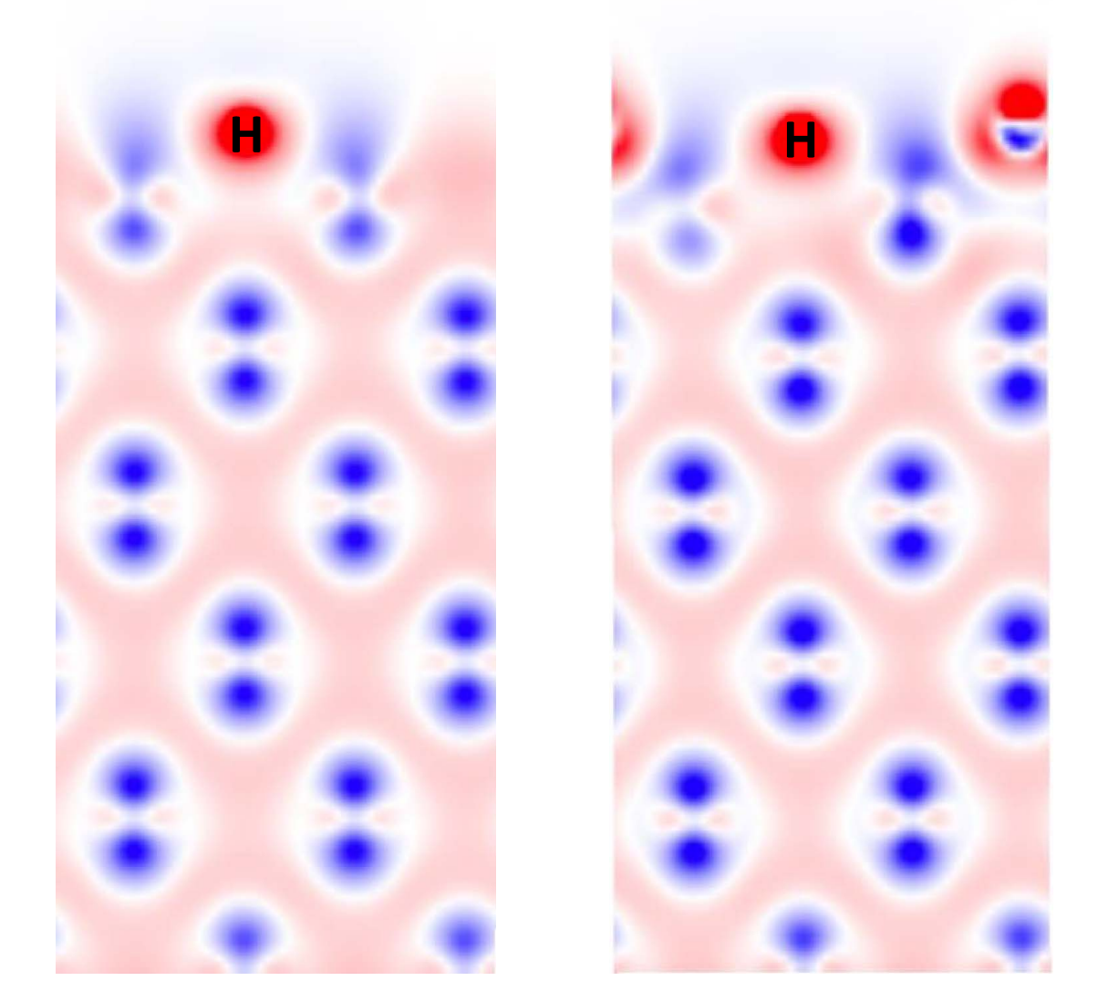
Y. Ferro et al 2023 Nucl. Fusion 63 036017

Length scale

Time scale

MD
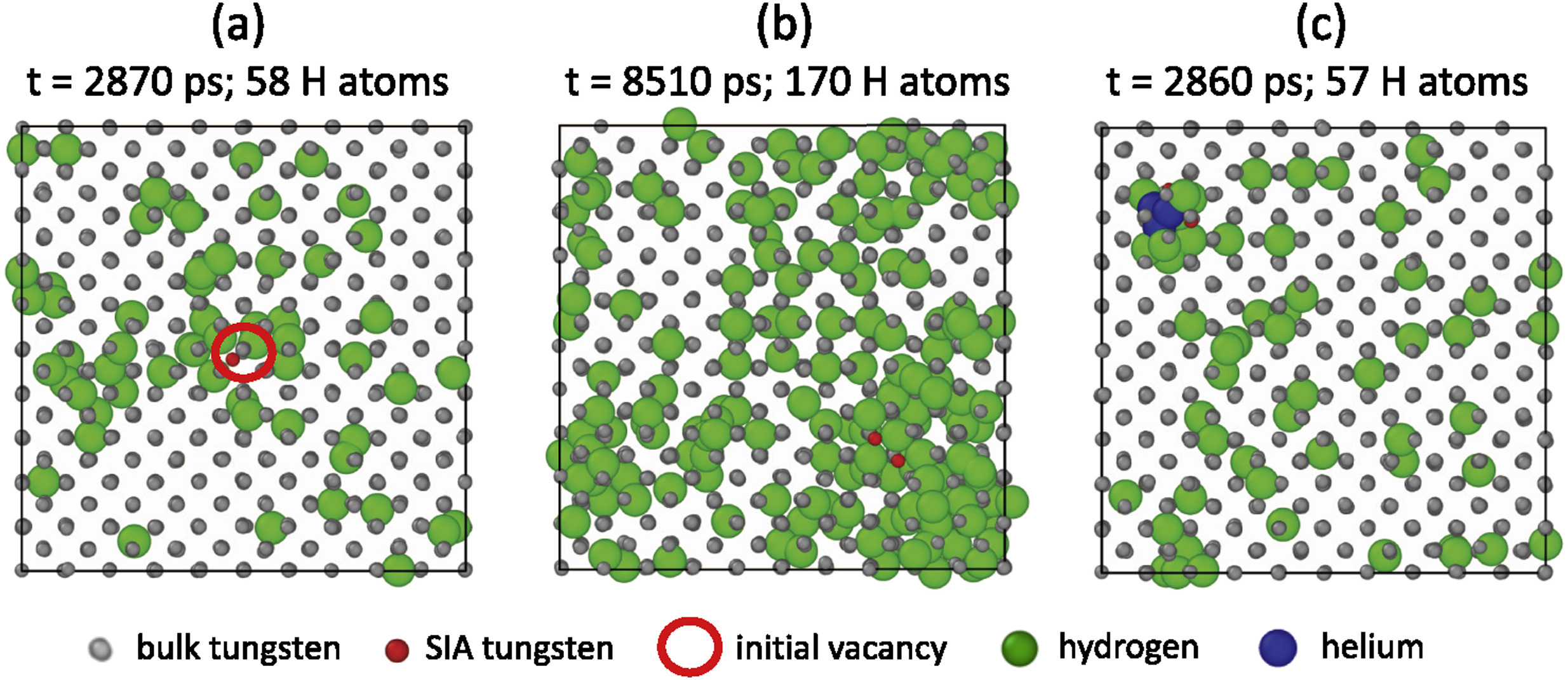
Length scale

Time scale

DFT

potentials

Multi-scale hydrogen transport

Component scale modelling
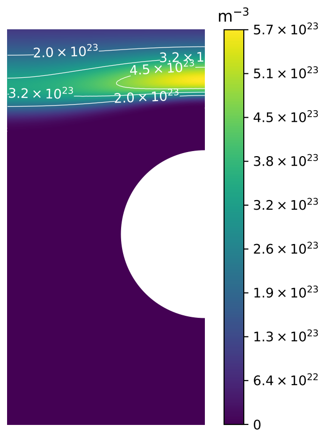
Length scale

Time scale

MD

DFT

D, S, other coeffs.

Multi-scale hydrogen transport

Length scale

Time scale

MD

DFT

Component scale modelling

Fuel cycle modelling
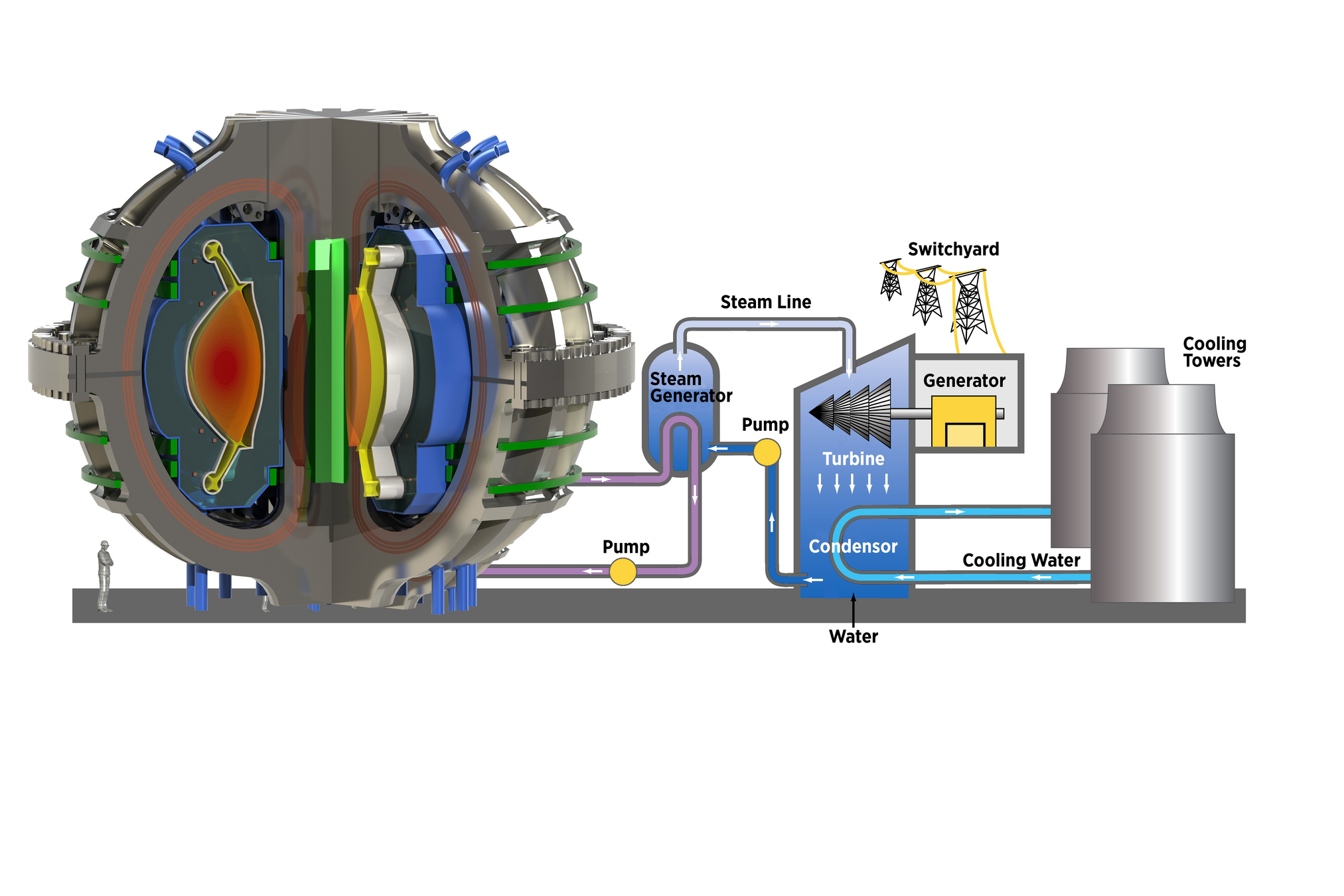
Residency times, fluxes, ...

Multi-scale hydrogen transport

Length scale

Time scale

MD

DFT

Component scale modelling

Fuel cycle modelling

Abstraction

Multi-scale hydrogen transport
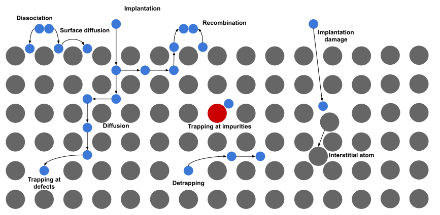
Tritium Transport in Materials


Diffusion

\varphi = - D \ \nabla c

\( \varphi\): diffusion flux

\( D \): diffusion coefficient

\( c \): mobile hydrogen concentration

\( S\): source term

Fick's 1st law of diffusion

\frac{\partial c}{\partial t} = - \nabla \cdot \varphi + S

Fick's 2nd law of diffusion

Trapping
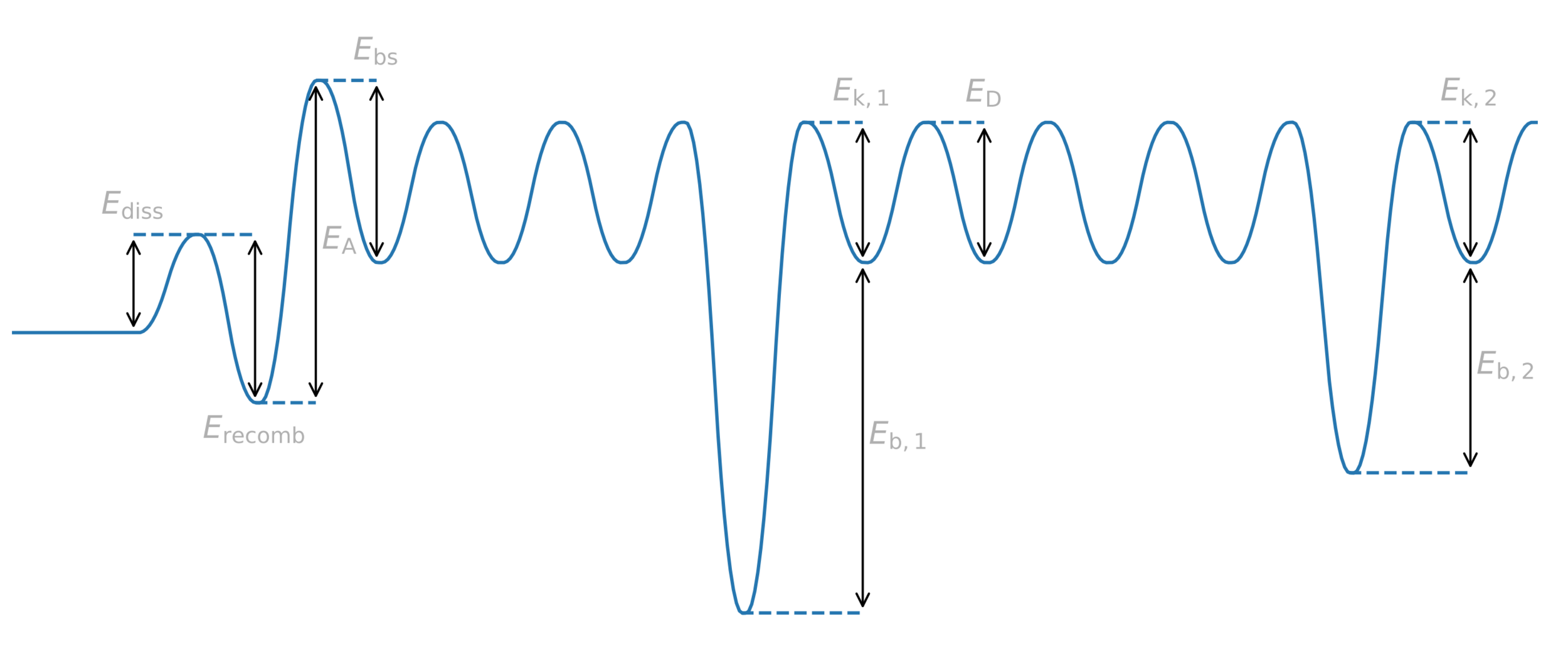
H

Potential energy

Distance

Diffusion barrier

Trap binding energy

Trapping energy

Common assumption:

\( E_k = E_D \)

Trapping

\mathrm{H} + [\ \ \ ]_\mathrm{trap} \ \substack{p \\[-1em] \longleftarrow\\[-1em] \longrightarrow \\[-1em] k} \ [\mathrm{H}]_\mathrm{trap}

0D

\frac{\partial c_\mathrm{t}}{\partial t} = -\frac{\partial c_\mathrm{m}}{\partial t} = k \ c_\mathrm{m} \ (n_\mathrm{trap,0} - c_\mathrm{t}) - p c_\mathrm{t}
c_\mathrm{m}
n_\mathrm{free \ trap}
c_\mathrm{t}

Total concentration of traps

McNabb & Foster Model

\frac{\partial c_\mathrm{m}}{\partial t} = \nabla \cdot (D \nabla c_\mathrm{m}) + S - \sum \frac{\partial c_\mathrm{t,i}}{\partial t}
\frac{\partial c_\mathrm{t, i}}{\partial t} = k_i \ c_\mathrm{m} \ (n_\mathrm{trap,i} - c_\mathrm{t}) - p_i c_\mathrm{t}

Particle implantation

Ziegler et al. 2010. Nuclear Instruments and Methods in Physics Research Section B: Beam Interactions with Materials and Atoms, 268 (11): 1818–23. https://doi.org/10.1016/j.nimb.2010.02.091.

Implantation range
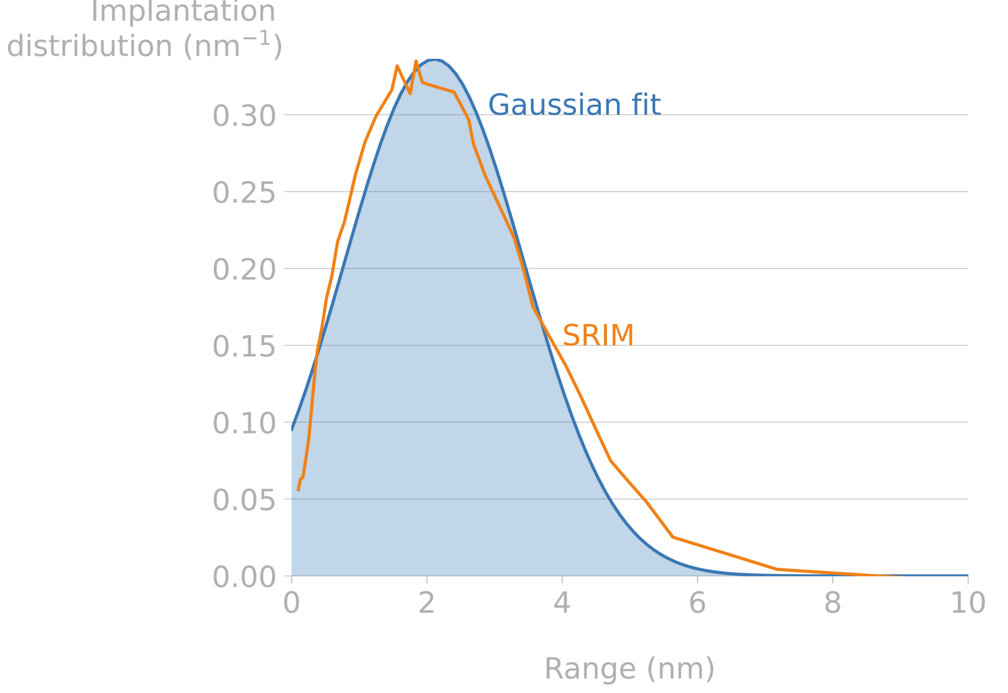
Implantation range & width and reflection coefficient can be computed with SRIM, SDTRIM...

Mutzke et al, SDTrimSP Version 6.00 2019

S = (1-r) \ \Gamma_\mathrm{incident} \ f(x)

\(\Gamma_\mathrm{incident} \): incident flux (particle/m2/s)

\( f(x) \): Gaussian distribution (/m)

\(r \): reflection coefficient

or

Surface effects

H2 molecules

Metal lattice

Surface effects

\varphi_\mathrm{dissociation} = K_\mathrm{d} \ P

Dissociation coefficient (H/m2/s/Pa)

Partial pressure of H (Pa)

Adsorbed H

Metal lattice

Surface effects

\varphi_\mathrm{dissociation} = K_\mathrm{d} \ P
\varphi_\mathrm{recombination} = K_\mathrm{r} \ c^2

Metal lattice

Recombination coefficient (m4/s)

Concentration (H/m3)

Surface effects

\varphi_\mathrm{dissociation} = K_\mathrm{d} \ P
\varphi_\mathrm{recombination} = K_\mathrm{r} \ c^2

Metal lattice

\varphi_\mathrm{net} = \varphi_\mathrm{dissociation} - \varphi_\mathrm{recombination}

Waelbroeck model

Surface effects

\varphi_\mathrm{dissociation} = K_\mathrm{d} \ P
\varphi_\mathrm{recombination} = K_\mathrm{r} \ c^2

Metal lattice

At equilibrium:

\varphi_\mathrm{net} = 0
c = \sqrt{\frac{K_\mathrm{d}}{K_\mathrm{r}}} \ \sqrt{P}
\varphi_\mathrm{net} = \varphi_\mathrm{dissociation} - \varphi_\mathrm{recombination}
c = K_S \ \sqrt{P}

Sievert's law of solubility

Surface effects

\varphi_\mathrm{dissociation} = K_\mathrm{d} \ P
\varphi_\mathrm{recombination} = K_\mathrm{r} \ c^1

Non-metallic liquid

At equilibrium:

\varphi_\mathrm{net} = 0
c = \frac{K_\mathrm{d}}{K_\mathrm{r}} \ P
\varphi_\mathrm{net} = \varphi_\mathrm{dissociation} - \varphi_\mathrm{recombination}
c = K_H \ P

Henry's law of solubility

Interfaces

Material 1

Material 2

Case 1:

Metal-Metal

- D_1 \nabla c_1 = - D_2 \nabla c_2
P = \left( \frac{c}{K_S} \right) ^2
\left( \frac{c_1}{K_{S,1}} \right)^2 =\left( \frac{c_2}{K_{S,2}} \right)^2

Sievert's law

Flux continuity

Conservation of chemical potential

Interfaces

Material 1

Material 2

Case 2:

Non metal-non metal

- D_1 \nabla c_1 = - D_2 \nabla c_2
P = \frac{c}{K_H}
\frac{c_1}{K_{H,1}} = \frac{c_2}{K_{H,2}}

Henry's law

Flux continuity

Conservation of chemical potential

Interfaces

Material 1

Material 2

Case 3:

Metal-Non metal

- D_1 \nabla c_1 = - D_2 \nabla c_2
P = \left( \frac{c}{K_S} \right) ^2
\left( \frac{c_1}{K_{S,1}} \right)^2 = \frac{c_2}{K_{H,2}}

Sievert's law

P = \frac{c}{K_H}

Henry's law

\frac{\partial c_\mathrm{m}}{\partial t} = \nabla \cdot \varphi_\mathrm{diffusion} + S - \sum \frac{\partial c_\mathrm{t,i}}{\partial t}
\frac{\partial c_\mathrm{t, i}}{\partial t} = k_i \ c_\mathrm{m} \ (n_\mathrm{trap,i} - c_\mathrm{t}) - p_i c_\mathrm{t}

McNabb & Foster model

Challenges

  • Number of degrees of freedom
  • Interface discontinuities

Governing equations

- D_1 \nabla c_1 = - D_2 \nabla c_2
\left( \frac{c_1}{K_{1}} \right)^2 =\left( \frac{c_2}{K_{2}} \right)^{\{1,2\} }

We can solve these numerically

Component modelling

Experimental analysis

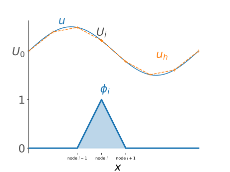
3 main numerical methods

Finite Difference Method (FDM)

Finite Element Method (FEM)

Finite Volume Method (FVM)

Let's not bother

\frac{\partial c }{\partial x} \approx \frac{c(x=x_{i+1}) - c(x=x_{i})}{x_{i+1} - x_{i}}
FESTIM today
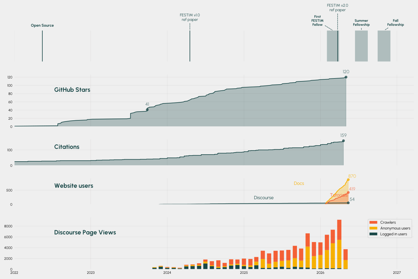
See more FESTIM stats:
festim-dev.github.io/pose

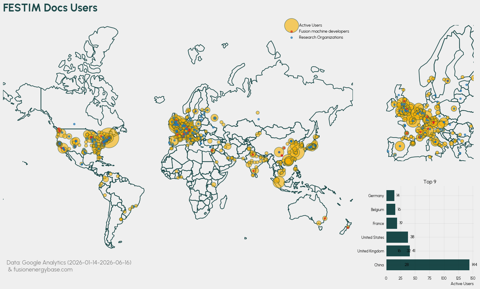
FESTIM is used worldwide

Docs users

Fusion machine developers

Research organisations

What changed in FESTIM2?

Upgrade from legacy-FEniCS to FEniCSx

  Before

  • Change of variable required - did not scale well
  • Single solver method available
  • No submesh coupling
  • Limited mesh element types


 Now

  • Mixed-domain: no substitution needed
  • Multiple solver methods (Penalty, Nitches)
  • Submesh coupling: 1D to 2D problems
  • Mixed topology meshes
  • Improved parallel I/O 


~11x faster

  Before

  • Monolithic approach
  • Change of variable required
    • Poor scaling
  • Little control over interface equations
  • Adding advection was tricky

  Now

  • Mixed-domain: no substitution needed
  • No change of variable needed
  • Improved performance
  • Full control over interface conditions
  • Very suitable for multi-physics 


Multi-material handling

Multi-species and Reactions

  Before

  • Single mobile species only
  • No multi-isotope support
  • No multi-occupancy trapping
  • Rigid trapping reactions

  Now

  • Arbitrary species
    • Multi-isotope
    • Multi-occupancy trapping
    • Defect diffusion
  • Flexible reactions
  • Bulk and surface reactions


The mixed formulation is great for multiphysics

velocity, temperature, turbulent viscosity...

tritium production

Heat source

Temperature

Neutronics

Thermo-hydraulics

Tritium transport
Examples
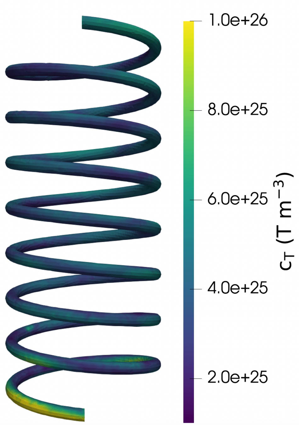
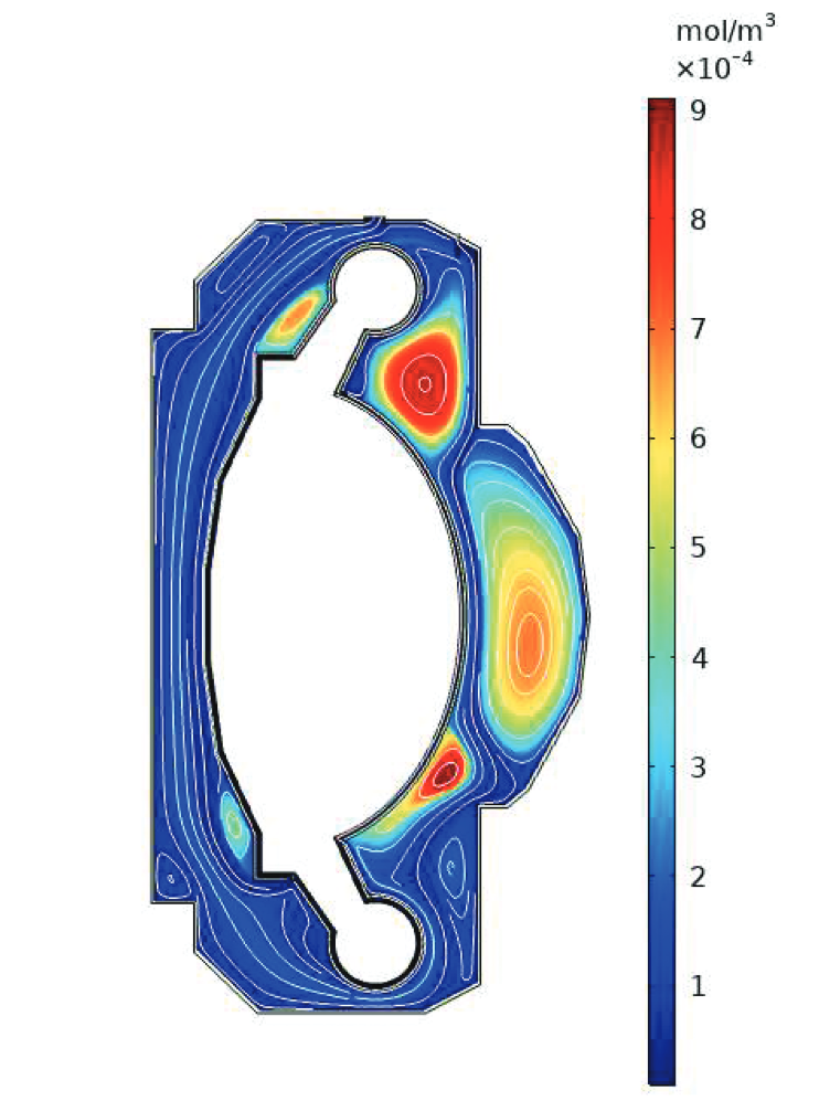
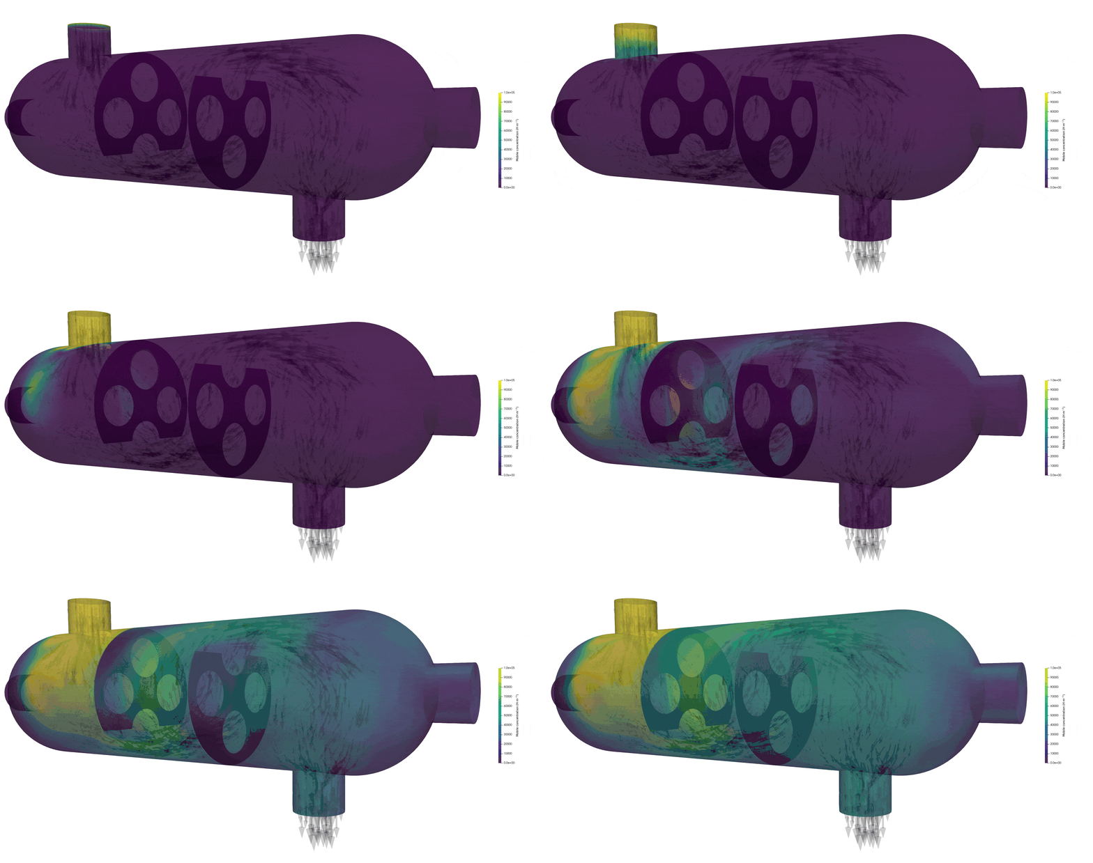
Using FESTIM for estimating tritium contamination in a heat exchanger
ARC Breeding Blanket

ARC blanket geometry

T source

Heat source

Velocity

Temperature

Turbulent viscosity

Tritium concentration

TDS analysis: codeposits

  • Simulation of W codeposited layers
     
  • Influence of partial pressure
     
  • 10 different traps!

Thank you for your attention!

Any questions?
FESTIM Fellowship programme commenced in 2026

"Even though it's quite nice to be the FESTIM v2 expert on site (!!!), I would absolutely recommend the programme to my colleagues."

First FESTIM fellow - Tez Orr (UKAEA)


Hands-on-learning - Tez worked directly with the dev team on UKAEA cases and fixed a bug in v2.0


Immediate impact  - Became UKAEA's resident FESTIM expert, contributing to both the LIBRTI and STEP programmes


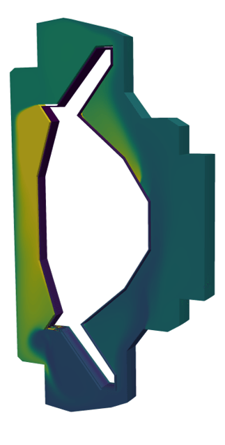
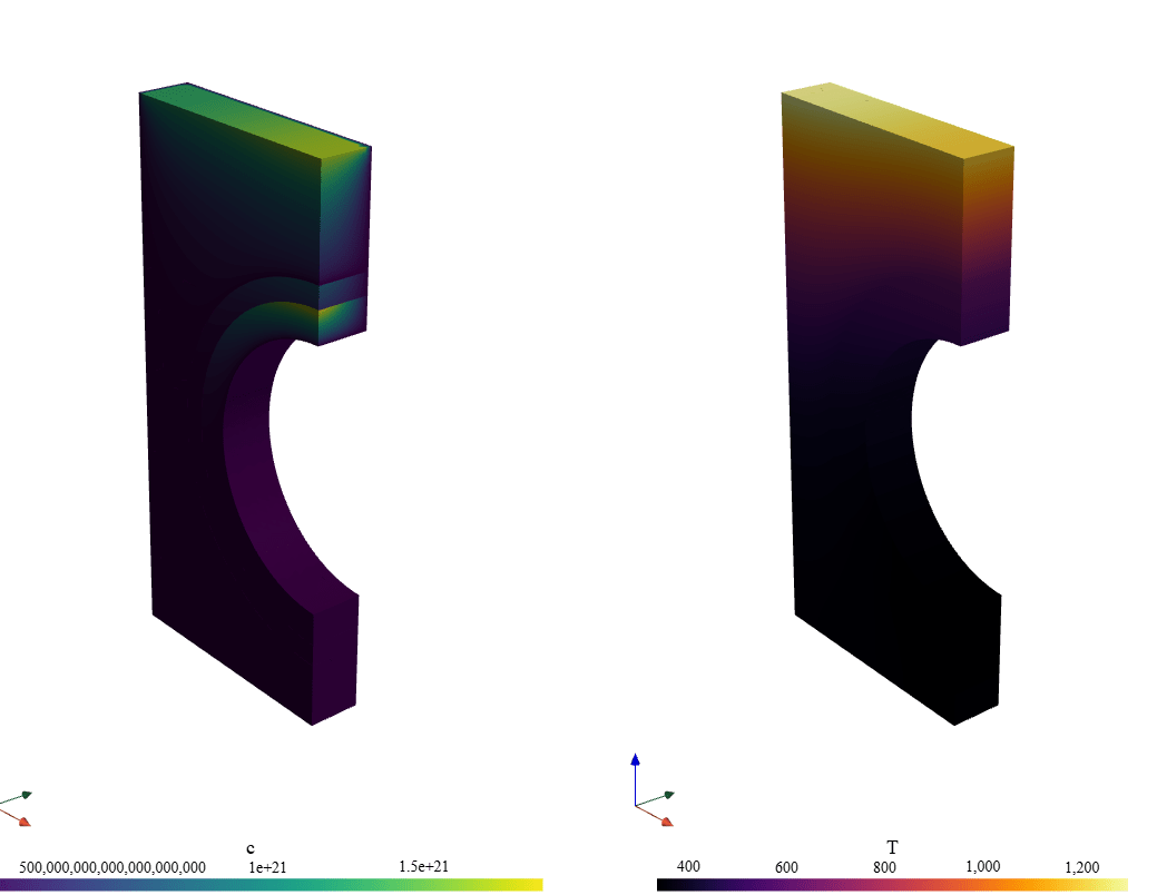
Monoblock

CAD based simulations

Read a mesh from GMSH

mesh_data = gmshio.read_from_msh(
    "gmsh/mesh3D.msh", MPI.COMM_WORLD, 0, gdim=3
)
mesh = mesh_data.mesh

facet_tags = mesh_data.facet_tags

cell_tags = mesh_data.cell_tags

Can also import meshes from other sources thanks to io4dolfinx

Heat transfer simulation

Run heat conduction simulation

heat_transfer_problem = F.HeatTransferProblem()

...

heat_flux_top = F.HeatFluxBC(subdomain=top_surface, value=10e6)

convective_flux_coolant = F.HeatFluxBC(
    subdomain=cooling_surface, value=lambda T: h_convective * (T_coolant - T)
)

...

heat_transfer_problem.run()
10^6 \ \mathrm{W/m^2}

Convective cooling

H transport problem

Pass the temperature field to the H transport problem

my_model = F.HydrogenTransportProblemDiscontinuous()

my_model.temperature = heat_transfer_problem.u

my_model.method_interface = "penalty"

my_model.subdomains = all_subdomains

H = F.Species("H", subdomains=my_model.volume_subdomains)
my_model.species = [H]

my_model.mesh = mesh

my_model.surface_to_volume = {
    top_surface: tungsten_volume,
    cooling_surface: cucrzr_volume,
    poloidal_gap_w: tungsten_volume,
    poloidal_gap_cu: copper_volume,
    poloidal_gap_cucrzr: cucrzr_volume,
    toroidal_gap: tungsten_volume,
    bottom: tungsten_volume,
}

penalty_term = 1e20
my_model.interfaces = [
    F.Interface(
        id=16, subdomains=(tungsten_volume, copper_volume), penalty_term=penalty_term
    ),
    F.Interface(
        id=17, subdomains=(copper_volume, cucrzr_volume), penalty_term=penalty_term
    ),
]

import ufl

# Plasma implantation flux BC
phi = 1.61e22
R_p = 9.52e-10
implantation_flux_top = F.FixedConcentrationBC(
    subdomain=top_surface,
    value=lambda T: phi * R_p / (tungsten.D_0 * ufl.exp(-tungsten.E_D / F.k_B / T)),
    species=H,
)

# Instantaneous molecular recombination flux BCs at all other surfaces (fixed concentration of 0)
recombination_fluxes = [
    F.FixedConcentrationBC(subdomain=surf, value=0, species=H)
    for surf in [
        toroidal_gap,
        bottom,
        poloidal_gap_w,
        poloidal_gap_cu,
        poloidal_gap_cucrzr,
        cooling_surface,
    ]
]

my_model.boundary_conditions = [implantation_flux_top] + recombination_fluxes

exports = {
    "poloidal_gap_cu_flux": F.SurfaceFlux(surface=poloidal_gap_cu, field=H),
    "poloidal_gap_cucrzr_flux": F.SurfaceFlux(surface=poloidal_gap_cucrzr, field=H),
    "poloidal_gap_w_flux": F.SurfaceFlux(surface=poloidal_gap_w, field=H),
    "toroidal_gap_flux": F.SurfaceFlux(surface=toroidal_gap, field=H),
    "bottom_flux": F.SurfaceFlux(surface=bottom, field=H),
    "inventory_w": F.TotalVolume(field=H, volume=tungsten_volume),
    "inventory_cu": F.TotalVolume(field=H, volume=copper_volume),
    "inventory_cucrzr": F.TotalVolume(field=H, volume=cucrzr_volume),
}


my_model.exports = list(exports.values())

my_model.settings = F.Settings(
    atol=1e-8,
    rtol=1e-10,
    transient=False,
    max_iterations=10,
)

my_model.initialise()
my_model.run()

Implantation from plasma

c = 0

Examples: multi-species framework

Multi-species

H = F.Species("H")

my_model.species = [H]

Defining species

\mathrm{H}

Multi-species

H = F.Species("H")
D = F.Species("D")


my_model.species = [H, D]
\mathrm{H}, \mathrm{D}

Defining species

Multi-species

H = F.Species("H")
empty_traps = F.Species("empty", mobile=False)
trapped_H = F.Species("trapped_H", mobile=False)


my_model.species = [H, empty_traps, trapped_H]

Adding a reaction

\mathrm{H} + [\ ] \xrightleftharpoons[p]{k} [\mathrm{H}]
trapping = F.Reaction(
	reactant=[H, empty_traps],
    product=[trapped_H],
    k_0=...,
    E_k=...,
    p_0=...,
    E_p=...,
)


my_model.reactions = [trapping]

Multi-species

H = F.Species("H")
empty_traps = F.Species("empty", mobile=True)
trapped_H = F.Species("trapped_H", mobile=False)


my_model.species = [H, empty_traps, trapped_H]

Mobile traps?

\mathrm{H} + [\ ] \xrightleftharpoons[p]{k} [\mathrm{H}]
trapping = F.Reaction(
	reactant=[H, empty_traps],
    product=[trapped_H],
    k_0=...,
    E_k=...,
    p_0=...,
    E_p=...,
)


my_model.reactions = [trapping]

Multi-species

H = F.Species("H")
empty_traps = F.Species("empty", mobile=False)
empty_traps2 = F.Species("empty2", mobile=False)
trapped_H = F.Species("trapped_H", mobile=False)
trapped_H2 = F.Species("trapped_H2", mobile=False)

my_model.species = [
  H, empty_traps, trapped_H,
  empty_traps2, trapped_H2
]

2 traps

\mathrm{H} + [\ ] \xrightleftharpoons[p]{k} [\mathrm{H}]
trapping = F.Reaction(
	reactant=[H, empty_traps],
    product=[trapped_H],
	...
)

trapping2 = F.Reaction(
	reactant=[H, empty_traps2],
    product=[trapped_H2],
	...
)


my_model.reactions = [trapping, trapping2]
\mathrm{H} + [\ ]_2 \xrightleftharpoons[p_2]{k_2} [\mathrm{H}]_2

Multi-species

H = F.Species("H")
D = F.Species("D")
empty_traps = F.Species("empty", mobile=False)
trapped_H = F.Species("trapped_H", mobile=False)
trapped_D = F.Species("trapped_D", mobile=False)


my_model.species = [
  H, D, empty_traps,
  trapped_H, trapped_D
]

1 trap, 2 isotopes

\mathrm{H} + [\ ] \xrightleftharpoons[p]{k} [\mathrm{H}]
trapping = F.Reaction(
	reactant=[H, empty_traps],
    product=[trapped_H],
	...
)

trapping2 = F.Reaction(
	reactant=[D, empty_traps],
    product=[trapped_D],
	...
)


my_model.reactions = [trapping, trapping2]
\mathrm{D} + [\ ] \xrightleftharpoons[p]{k} [\mathrm{D}]

Multi-species

H = F.Species("H")
empty_traps = F.Species("empty", mobile=False)
trapped_H = F.Species("trapped_H", mobile=False)
trapped_H2 = F.Species("trapped_H2", mobile=False)

my_model.species = [
  H, empty_traps,
  trapped_H, trapped_H2
]

Multi-occupancy trapping

\mathrm{H} + [\ ] \xrightleftharpoons[p]{k} [\mathrm{H}]
trapping = F.Reaction(
	reactant=[H, empty_traps],
    product=[trapped_H],
	...
)

trapping2 = F.Reaction(
	reactant=[H, empty_traps2],
    product=[trapped_H2],
	...
)


my_model.reactions = [trapping, trapping2]
\mathrm{H} + [\mathrm{H}] \xrightleftharpoons[p]{k} [\mathrm{HH}]

Multi-species

A = F.Species("A")
B = F.Species("B")
C = F.Species("C")
D = F.Species("D")

my_model.species = [A, B, C, D]
\mathrm{A} + \mathrm{B} \xrightleftharpoons[p]{k} \mathrm{C} + \mathrm{D}

"Species" can be anything...

Multi-species

A = F.Species("A")
B = F.Species("B")
C = F.Species("C")
D = F.Species("D")

my_model.species = [A, B, C, D]
\mathrm{A} + \mathrm{B} \xrightleftharpoons[p]{k} \mathrm{C} + \mathrm{D}
reac = F.Reaction(
    reactant=[A, B],
    product=[C, D],
    ...
)

Arbitrary numbers of reactants and products

Multi-species

A = F.Species("A")
B = F.Species("B")


my_model.species = [A, B]
\mathrm{A} + \mathrm{B} \xrightarrow{k} \emptyset
reac = F.Reaction(
    reactant=[A, B],
    product=[],
    ...
)

Arbitrary numbers of reactants and products

Can be used for:

  • Vacancy-Interstitial anhiliation
  • Radioactive decay
  • Defect annealing
  • ...

Multi-species

H = F.Species("H")


my_model.species = [H]

reac = F.SurfaceReactionBC(
    reactant=[H, H],
    pressure=10,
    ...
)

my_model.boundary_conditions = [reac]

Surface reactions

2 \mathrm{H} \xrightleftharpoons[K_d]{K_r} \mathrm{H}_2

Soon: support for dynamically computed gas pressures (enclosures)

Examples: Multiphysics coupling


Integrate results from external solvers into FESTIM

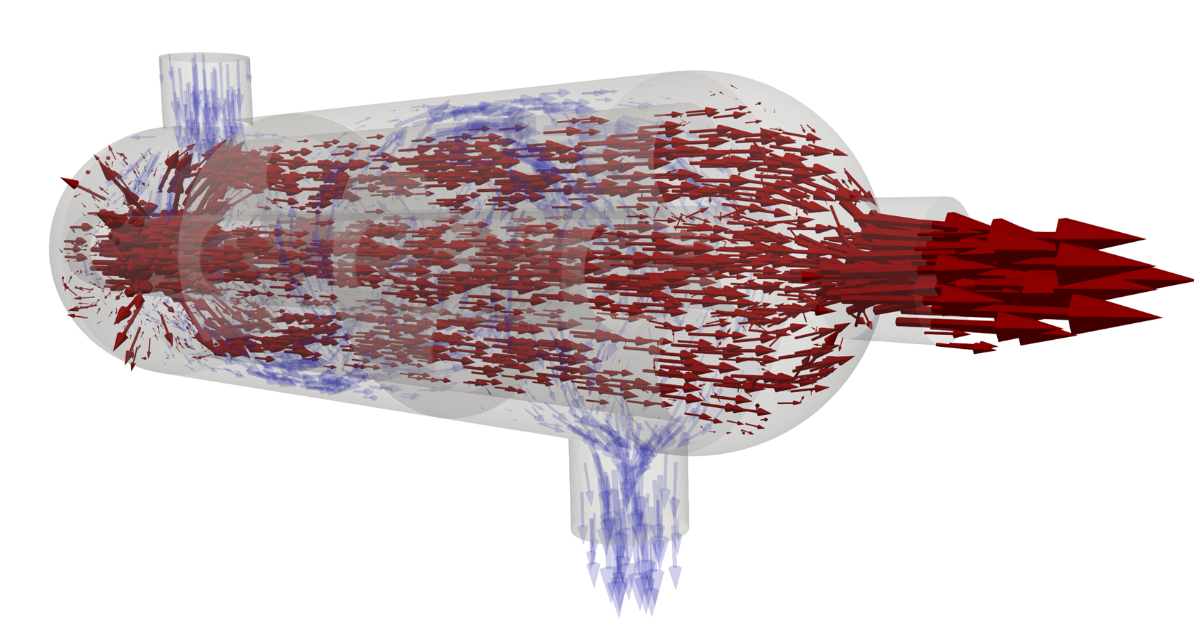
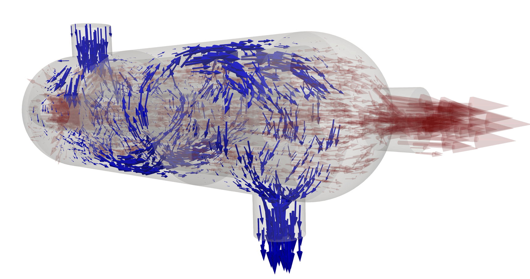
Coupling CFD to FESTIM using foam2dolfinx

Using foam2dolfinx we can pass velocity fields calculated from OpenFOAM to FESTIM

Reading OpenFOAM data using foam2dolfinx

from foam2dolfinx import OpenFOAMReader

reader = OpenFOAMReader(filename="my_foam_case.foam", cell_type=10)


# read fields
u = reader.create_dolfinx_function_with_point_data(t=100, name="U")


# read mesh
foam_mesh = reader.dolfinx_meshes_dict["default"]


# read meshtags
facet_mt = reader.create_facet_meshtags()
volume_mt = reader.create_cell_meshtags()

Read a local OpenFOAM case file


  • Specify time stamp of data
  • Can extract any field type
  • Extract dolfinx mesh
  • Extract meshtags

Tets

Hexes

Support for:


Reading and writing using io4dolfinx

import io4dolfinx

checkpoint_file = Path("sim_checkpoint.bp")

io4dolfinx.write_mesh(checkpoint_file, msh)
io4dolfinx.write_function(checkpoint_file, u, time=100, name="U")
io4dolfinx.write_meshtags(checkpoint_file, msh, facet_mt, meshtag_name="facet_tags")
io4dolfinx.write_meshtags(checkpoint_file, msh, cell_mt, meshtag_name="cell_tags")

..

msh = io4dolfinx.read_mesh(checkpoint_file, COMM)
facet_mt = io4dolfinx.read_meshtags(checkpoint_file, msh, meshtag_name="facet_tags")
cell_mt = io4dolfinx.read_meshtags(checkpoint_file, msh, meshtag_name="cell_tags")

gdim = msh.geometry.dim
el = basix.ufl.element("Lagrange", msh.topology.cell_name(), 1, shape=(gdim,))
w = fem.Function(fem.functionspace(msh, el), name="U")
io4dolfinx.read_function(checkpoint_file, u, time=100, name="U")

Using OpenFOAM data in FESTIM

...


my_model.mesh = foam_mesh

my_model.surface_meshtags = facet_meshtags
my_model.volume_meshtags = cell_meshtags


...


my_model.advection_terms = [
  F.AdvectionTerm(velocity=u, species=H, subdomain=fluid)
]

Pass mesh and meshtags to FESTIM


Pass velocity field using F.AdvectionTerm()


Adding advection to FESTIM means adding a term in the formulation

\frac{\partial c}{\partial t} = \nabla\cdot(D \nabla c) + S
- \nabla \cdot ( \mathbf{u} c)

Coupling neutronics to FESTIM using openmc2dolfinx

Using openmc2dolfinx we can pass fields calculated from OpenMC to FESTIM

from openmc2dolfinx import UnstructuredMeshReader, StructuredMeshReader

# UnstructuredMeshReader for tets
reader = UnstructuredMeshReader(filename="out.vtk")

# StructuredMeshReader for hexs
reader = StructuredMeshReader(filename="out.vtk")

# read fields
source_from_openmc = reader.create_dolfinx_function(name="mean")

Reading OpenMC data using openmc2dolfinx

Read .vtk file produced by OpenMC


  • Extract any mesh tally:
    • ​Tritium production
    • Heat generation
    • He production ...

Tets

Hexes

Support for:


...


my_model.sources = [
  F.ParticleSource(value=source_from_openmc, species=T, subdomain=volume)
]


...

Using OpenMC data in FESTIM

Input into FESTIM as a source term

Examples: FESTIM in the loop

Integrate FESTIM in complex workflows

Machine Learning with FESTIM

1. Parametric FESTIM model

2. Produce training data

3. Train surrogate/emulator

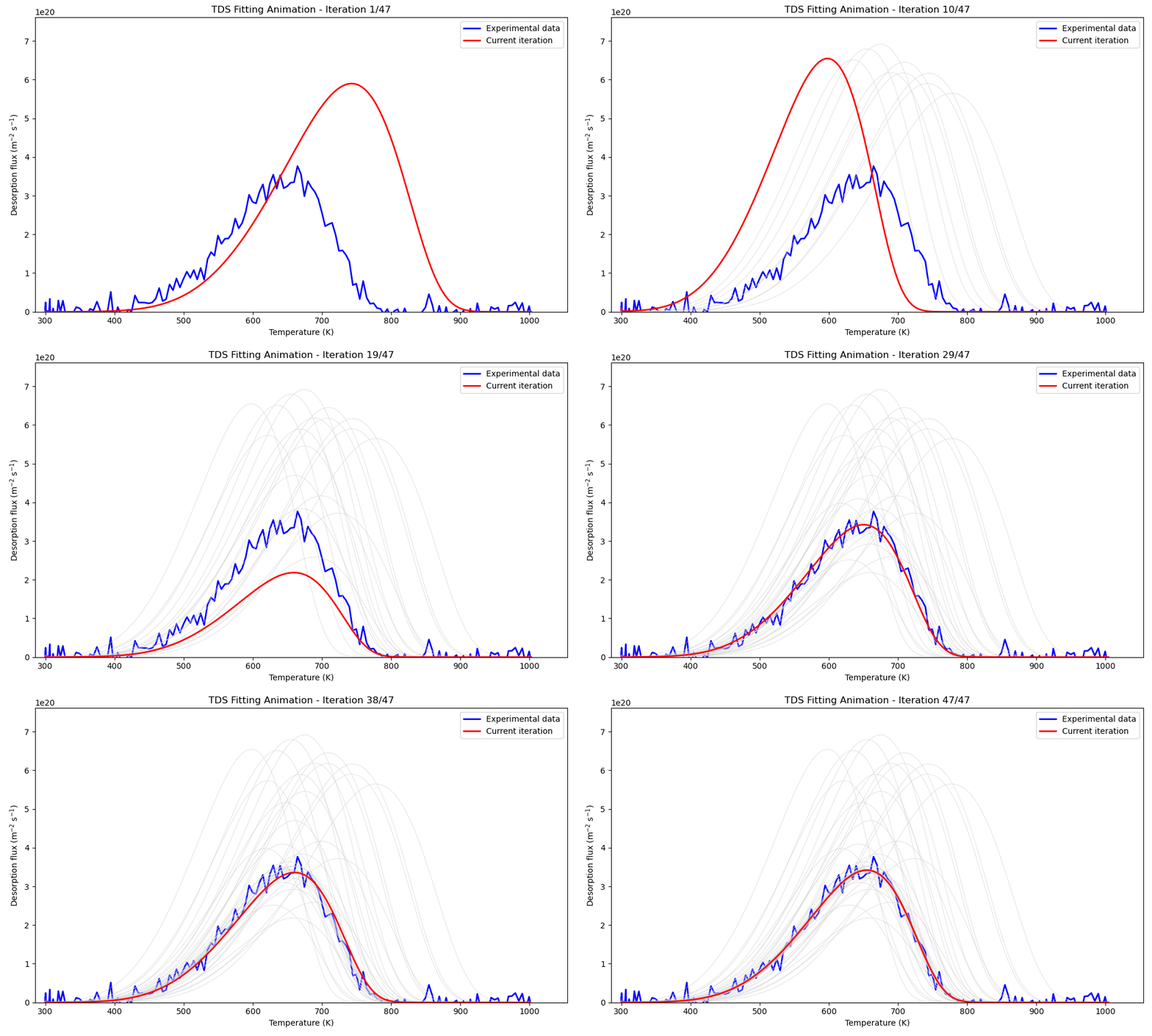
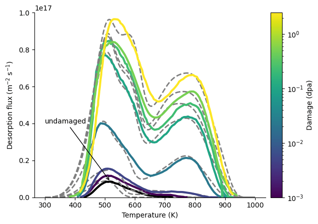
Parametric optimisation with FESTIM

Goal: find the trapping parameters to reproduce an experimental thermo-desorption spectrum

Integrating FESTIM with fuel cycle models

PathView/PathSim: a python package for system modelling

pathsim.org


Can be seamlessly coupled with FESTIM for multi-fidelity fuel cycle simulations

UKAEA FESTIM workshop 2026

By Remi Delaporte-Mathurin
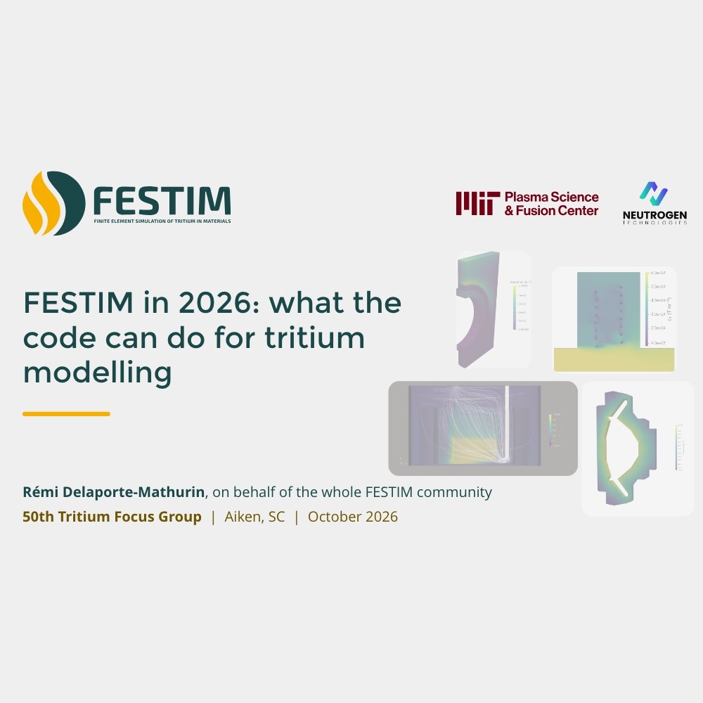
UKAEA FESTIM workshop 2026

  • 78