workshop materials


June 2026

Kaelyn Dunnell  -  Tez Orr

Agenda

Day 1 – Saturday, 21 June 2025


08:15 – 09:15  General Introduction, tritium in fusion – Remi Delaporte-Mathurin


09:15 – 09:30  Coffee Break


09:30 – 10:30  Modelling hydrogen transport: reactor scale and fuel cycle – Samuele Meschini

10:30 – 11:30  Modelling hydrogen transport: component to reactor scale – Remi Delaporte-Mathurin

11:30 – 12:30  Modelling hydrogen transport: atomistic scale – Stephen Lam


12:30 – 13:30  Lunch
 

13:30 – 15:30  Experimental techniques and material characterization – Thomas Fuerst, Hans Gietl

15:30 – 15:45  Coffee break

15:45 – 17:00  Q&A


Day 2 – Sunday, 22 June 2025
 

08:30 – 16:00  FESTIM workshop – Remi Delaporte-Mathurin, James Dark

Round of introductions

Introuction - Dr. Remi Delaporte-Mathurin

  • 2022-today: Researcher at the Plasma Science and Fusion Center, MIT
     
  • 2018-2019: Ph.D. French Atomic Energy Authority (CEA Cadarache) and University Sorbonne Paris Nord
     
  • 2017: CEA Cadarache, IRFM, apprentice
     
  • 2016: UK Atomic Energy Authority
     
  • 2012-2018: M.Sc. Thermal Engineering and Energy Sciences

Joint European Torus (JET), Culham, UK

DFT

Multi-scale hydrogen transport

Y. Ferro et al 2023 Nucl. Fusion 63 036017

Length scale

Time scale

MD

Length scale

Time scale

DFT

potentials

Multi-scale hydrogen transport

Component scale modelling

Length scale

Time scale

MD

DFT

D, S, other coeffs.

Multi-scale hydrogen transport

Length scale

Time scale

MD

DFT

Component scale modelling

Fuel cycle modelling

Residency times, fluxes, ...

Multi-scale hydrogen transport

Length scale

Time scale

MD

DFT

Component scale modelling

Fuel cycle modelling

Abstraction

Multi-scale hydrogen transport

Question time!

Tritium transport theory

Hydrogen transport in metals

Diffusion

Even more particles

continuity approximation

Single particle

Random walk

Many particles

Diffusion

\varphi = - D \ \nabla c

\( \varphi \): diffusion flux

\( D \): diffusion coefficient

\( c \): mobile hydrogen concentration

Fick's 1st law of diffusion

Diffusion

\varphi = - D \ \nabla c

\( \varphi\): diffusion flux

\( D \): diffusion coefficient

\( c \): mobile hydrogen concentration

\( S\): source term

Fick's 1st law of diffusion

\frac{\partial c}{\partial t} = - \nabla \cdot \varphi + S

Fick's 2nd law of diffusion

Diffusion

\varphi = - D \ \left( \nabla c + \frac{Q\ c}{R \ T^2} \ \nabla{T} - \frac{c \ V_H}{R \ T} \nabla \sigma \right)

\( \varphi\): diffusion flux

\( D \): diffusion coefficient

\( c \): mobile hydrogen concentration

\( S\): source term

Soret effect (or thermophoresis)

Stress assisted diffusion

Particle implantation

Ziegler et al. 2010. Nuclear Instruments and Methods in Physics Research Section B: Beam Interactions with Materials and Atoms, 268 (11): 1818–23. https://doi.org/10.1016/j.nimb.2010.02.091.

Implantation range

Implantation range & width and reflection coefficient can be computed with SRIM, SDTRIM...

Mutzke et al, SDTrimSP Version 6.00 2019

Particle implantation

S = (1-r) \ \Gamma_\mathrm{incident} \ f(x)

\(\Gamma_\mathrm{incident} \): incident flux (particle/m2/s)

\( f(x) \): Gaussian distribution (/m)

\(r \): reflection coefficient

Surface effects

H2 molecules

Metal lattice

Surface effects

\varphi_\mathrm{dissociation} = K_\mathrm{d} \ P

Dissociation coefficient (H/m2/s/Pa)

Partial pressure of H (Pa)

Adsorbed H

Metal lattice

Surface effects

\varphi_\mathrm{dissociation} = K_\mathrm{d} \ P
\varphi_\mathrm{recombination} = K_\mathrm{r} \ c^2

Metal lattice

Recombination coefficient (m4/s)

Concentration (H/m3)

Surface effects

\varphi_\mathrm{dissociation} = K_\mathrm{d} \ P
\varphi_\mathrm{recombination} = K_\mathrm{r} \ c^2

Metal lattice

\varphi_\mathrm{net} = \varphi_\mathrm{dissociation} - \varphi_\mathrm{recombination}

Waelbroeck model

Surface effects

\varphi_\mathrm{dissociation} = K_\mathrm{d} \ P
\varphi_\mathrm{recombination} = K_\mathrm{r} \ c^2

Metal lattice

At equilibrium:

\varphi_\mathrm{net} = 0
c = \sqrt{\frac{K_\mathrm{d}}{K_\mathrm{r}}} \ \sqrt{P}
\varphi_\mathrm{net} = \varphi_\mathrm{dissociation} - \varphi_\mathrm{recombination}
c = K_S \ \sqrt{P}

Sievert's law of solubility

Surface effects

\varphi_\mathrm{dissociation} = K_\mathrm{d} \ P
\varphi_\mathrm{recombination} = K_\mathrm{r} \ c^1

Non-metallic liquid

At equilibrium:

\varphi_\mathrm{net} = 0
c = \frac{K_\mathrm{d}}{K_\mathrm{r}} \ P
\varphi_\mathrm{net} = \varphi_\mathrm{dissociation} - \varphi_\mathrm{recombination}
c = K_H \ P

Henry's law of solubility

Interfaces

Material 1

Material 2

Interfaces

Partial pressure and flux are continuous

Material 1

Material 2

Interfaces

Material 1

Material 2

Case 1:

Metal-Metal

- D_1 \nabla c_1 = - D_2 \nabla c_2
P = \left( \frac{c}{K_S} \right) ^2
\left( \frac{c_1}{K_{S,1}} \right)^2 =\left( \frac{c_2}{K_{S,2}} \right)^2

Sievert's law

Interfaces

Material 1

Material 2

Case 2:

Non metal-non metal

- D_1 \nabla c_1 = - D_2 \nabla c_2
P = \frac{c}{K_H}
\frac{c_1}{K_{H,1}} = \frac{c_2}{K_{H,2}}

Henry's law

Interfaces

Material 1

Material 2

Case 3:

Metal-Non metal

- D_1 \nabla c_1 = - D_2 \nabla c_2
P = \left( \frac{c}{K_S} \right) ^2
\left( \frac{c_1}{K_{S,1}} \right)^2 = \frac{c_2}{K_{H,2}}

Sievert's law

P = \frac{c}{K_H}

Henry's law

Interfaces

Material 1

Material 2

Steady state concentration profile

  • different diffusivities \(\rightarrow\) different concentration gradients
  • different solubilities \( \rightarrow \) concentration discontinuity

\(x\)

\(c\)

⚠️Very little experimental validation data for interfaces

Permeation barriers are low solubility, low duffisivity

Metal

Tritiated environment

"Clean" environment

Permeation

Permeation barrier

Permeation barriers are low solubility, low duffisivity

Pressure \(P\)

High gradient = high flux

Low gradient = low flux

c
c

Pressure \(P\)

Trapping

H

Trap = anything binding to H

  • vacancy
  • grain boundary
  • impurity
  • chemical reaction
  • ...

Trapping

H

Potential energy

Distance

Diffusion barrier

Energy barrier = activation energy

Trap binding energy

Trapping energy

Common assumption:

\( E_k = E_D \)

Trapping

\mathrm{H} + [\ \ \ ]_\mathrm{trap} \ \substack{p \\[-1em] \longleftarrow\\[-1em] \longrightarrow \\[-1em] k} \ [\mathrm{H}]_\mathrm{trap}

0D

\frac{\partial c_\mathrm{t}}{\partial t} = -\frac{\partial c_\mathrm{m}}{\partial t} = k \ c_\mathrm{m} \ n_\mathrm{free \ trap} - p c_\mathrm{t}
c_\mathrm{t}

Since \(n_\mathrm{trap} = n_\mathrm{free \ trap} + c_\mathrm{t}  \)

c_\mathrm{m}
n_\mathrm{free \ trap}

Trapping

\mathrm{H} + [\ \ \ ]_\mathrm{trap} \ \substack{p \\[-1em] \longleftarrow\\[-1em] \longrightarrow \\[-1em] k} \ [\mathrm{H}]_\mathrm{trap}

0D

\frac{\partial c_\mathrm{t}}{\partial t} = -\frac{\partial c_\mathrm{m}}{\partial t} = k \ c_\mathrm{m} \ (n_\mathrm{trap,0} - c_\mathrm{t}) - p c_\mathrm{t}
c_\mathrm{m}
n_\mathrm{free \ trap}
c_\mathrm{t}

Total concentration of traps

Trapping

0D

\frac{\partial c_\mathrm{t}}{\partial t} = -\frac{\partial c_\mathrm{m}}{\partial t} = k \ c_\mathrm{m} \ (n_\mathrm{trap,0} - c_\mathrm{t}) - p c_\mathrm{t}

With diffusion

and 

1 trap

\frac{\partial c_\mathrm{m}}{\partial t} = \nabla \cdot \left(D\nabla c_\mathrm{m} \right) + S - \frac{\partial c_\mathrm{t}}{\partial t}
\frac{\partial c_\mathrm{t}}{\partial t} = k \ c_\mathrm{m} \ (n_\mathrm{trap,0} - c_\mathrm{t}) - p c_\mathrm{t}

Trapping

N traps

\frac{\partial c_\mathrm{m}}{\partial t} = \nabla \cdot \left(D\nabla c_\mathrm{m} \right) + S - \sum \frac{\partial c_\mathrm{t,i}}{\partial t}
\frac{\partial c_\mathrm{t, 1}}{\partial t} = k_1 \ c_\mathrm{m} \ (n_\mathrm{trap,1} - c_\mathrm{t,1}) - p_1 c_\mathrm{t,1}
\frac{\partial c_\mathrm{t, 2}}{\partial t} = k_2 \ c_\mathrm{m} \ (n_\mathrm{trap,2} - c_\mathrm{t,2}) - p_2 c_\mathrm{t,2}
\frac{\partial c_\mathrm{t, 3}}{\partial t} = k_3 \ c_\mathrm{m} \ (n_\mathrm{trap,3} - c_\mathrm{t,3}) - p_3 c_\mathrm{t,3}

McNabb & Foster model

Trapping

Other models assume traps can hold more than one H

\mathrm{H} + [\ \ \ ]_\mathrm{trap} \ \substack{p_1 \\[-1em] \longleftarrow\\[-1em] \longrightarrow \\[-1em] k_1} \ [\mathrm{H}_1]_\mathrm{trap}
\mathrm{H} + [\mathrm{H}_1]_\mathrm{trap} \ \substack{p_2 \\[-1em] \longleftarrow\\[-1em] \longrightarrow \\[-1em] k_2} \ [\mathrm{H}_2]_\mathrm{trap}
\mathrm{H} + [\mathrm{H}_2]_\mathrm{trap} \ \substack{p_3 \\[-1em] \longleftarrow\\[-1em] \longrightarrow \\[-1em] k_3} \ [\mathrm{H}_3]_\mathrm{trap}
\frac{\partial c_\mathrm{m}}{\partial t} = \nabla \cdot \left(D\nabla c_\mathrm{m} \right) + S - \sum{k_{i} \ c_\mathrm{m} \ c_{\mathrm{t},i-1} - p_i c_{\mathrm{t},i}}
\frac{\partial c_{\mathrm{t},i}}{\partial t} = k_{i} \ c_\mathrm{m} \ c_{\mathrm{t},i-1} - p_i c_{\mathrm{t},i} - k_{i+1} \ c_\mathrm{m} \ c_{\mathrm{t},i} + p_{i+1} c_{\mathrm{t},i+1}

Many of these processes are thermally activated

Recombination

Dissociation

Absorption

Trapping 

Detrapping

Diffusion

Arrhenius law

X = X_0 \ \exp{\left(\frac{-E_X}{k_B \ T}\right)}

Pre-exponential factor

Activation energy (eV/H)

Temperature (K)

Boltzmann constant (eV/H/K)

k_B = 8.617\times 10^{-5} \ \mathrm{eV/H/K}

Arrhenius law

X = X_0 \ \exp{\left(\frac{-E_X}{R \ T}\right)}

Pre-exponential factor

Activation energy (J/mol)

Temperature (K)

Gas constant (J/mol/K)

k_B = 8.617\times 10^{-5} \ \mathrm{eV/H/K}
R = 8.314 \ \mathrm{J/mol/K}
\frac{E_D [eV/H]}{k_B} = \frac{E_D [J/mol]}{R}

Conversion:

Arrhenius law

X = X_0 \ \exp{\left(\frac{-E_X}{R \ T}\right)}

\( 1/T \) (1/K)

E_X > 0
E_X < 0

Arrhenius law

X = X_0 \ \exp{\left(\frac{-E_X}{R \ T}\right)}
\log{(X)} = \log{(X_0)} \ - \frac{E_X}{k_B \ T}
\log{(X)} = \log{(X_0)} \ - \frac{E_X}{k_B} \ \frac{1}{T}

Intercept

+ Slope

Y =

X

Arrhenius law

Arrhenius parameters:

  • Diffusivity
  • Solubility
  • Permeability
  • Recombination coeff.
  • Dissociation coeff.
  • Trapping rate
  • Detrapping rate

Component scale modelling

\frac{\partial c_\mathrm{m}}{\partial t} = \nabla \cdot \varphi_\mathrm{diffusion} + S - \sum \frac{\partial c_\mathrm{t,i}}{\partial t}
\frac{\partial c_\mathrm{t, i}}{\partial t} = k_i \ c_\mathrm{m} \ (n_\mathrm{trap,i} - c_\mathrm{t}) - p_i c_\mathrm{t}

McNabb & Foster model

Challenges

  • Number of degrees of freedom
  • Interface discontinuities

Governing equations

- D_1 \nabla c_1 = - D_2 \nabla c_2
\left( \frac{c_1}{K_{1}} \right)^2 =\left( \frac{c_2}{K_{2}} \right)^{\{1,2\} }

Let's solve the system analytically

\frac{\partial c_\mathrm{m}}{\partial t} = \nabla \cdot \left(D\nabla c_\mathrm{m} \right) + S - \sum \frac{\partial c_\mathrm{t,i}}{\partial t}
\frac{\partial c_\mathrm{t, i}}{\partial t} = k_i \ c_\mathrm{m} \ (n_\mathrm{trap,i} - c_\mathrm{t,i}) - p_i c_\mathrm{t,i}

Let's solve the system analytically

Simplification #1:    1D domain \(L\)

\frac{\partial c_\mathrm{m}}{\partial t} = \frac{\partial}{\partial x} \left(D \frac{\partial}{\partial x} c_\mathrm{m} \right) + S - \sum \frac{\partial c_\mathrm{t,i}}{\partial t}
\frac{\partial c_\mathrm{t, i}}{\partial t} = k_i \ c_\mathrm{m} \ (n_\mathrm{trap,i} - c_\mathrm{t,i}) - p_i c_\mathrm{t,i}

Let's solve the system analytically

Simplification #1:    1D domain \(L\)

Simplification #2:    1 material

\frac{\partial c_\mathrm{m}}{\partial t} = \frac{\partial}{\partial x} \left(D \frac{\partial}{\partial x} c_\mathrm{m} \right) + S - \sum \frac{\partial c_\mathrm{t,i}}{\partial t}
\frac{\partial c_\mathrm{t, i}}{\partial t} = k_i \ c_\mathrm{m} \ (n_\mathrm{trap,i} - c_\mathrm{t,i}) - p_i c_\mathrm{t,i}

Let's solve the system analytically

D, S, k, p, n = \mathrm{constants}

Simplification #1:    1D domain \(L=1\)

Simplification #2:    1 material

Simplification #3:

\frac{\partial c_\mathrm{m}}{\partial t} = D \frac{\partial^2 c_\mathrm{m}}{\partial x^2} + S - \sum \frac{\partial c_\mathrm{t,i}}{\partial t}
\frac{\partial c_\mathrm{t, i}}{\partial t} = k_\mathrm{i} \ c_\mathrm{m} \ (n_\mathrm{trap,i} - c_\mathrm{t,i}) - p_\mathrm{i} c_\mathrm{t,i}

Let's solve the system analytically

D, S, k, p, n = \mathrm{constants}

Simplification #1:    1D domain \(L\)

Simplification #2:    1 material

Simplification #3:

Simplification #4: Steady state 

0 = k_\mathrm{i} \ c_\mathrm{m} \ (n_\mathrm{trap,i} - c_\mathrm{t,i}) - p_\mathrm{i} c_\mathrm{t,i}
0 = D \frac{\partial^2 c_\mathrm{m}}{\partial x^2} + S

💡Tip

At steady state, the mobile concentration is independent of trapping

Let's solve the system analytically

0 = k_\mathrm{i} \ c_\mathrm{m} \ (n_\mathrm{trap,i} - c_\mathrm{t,i}) - p_\mathrm{i} c_\mathrm{t,i}
0 = D \frac{\partial^2 c_\mathrm{m}}{\partial x^2} + S
c_\mathrm{t,i} = \frac{n_\mathrm{trap,i}}{1+ \frac{p_\mathrm{i}}{k_\mathrm{i} \ c_\mathrm{m}}}

Oriani's model

Let's solve the system analytically

0 = D \frac{\partial^2 c_\mathrm{m}}{\partial x^2} + S
c_\mathrm{t,i} = \frac{n_\mathrm{trap,i}}{1+ \frac{p_\mathrm{i}}{k_\mathrm{i} \ c_\mathrm{m}}}
\frac{\partial^2 c_\mathrm{m}}{\partial x^2} = \frac{-S}{D}
\frac{\partial c_\mathrm{m}}{\partial x} = \frac{-S}{D} x + K_1
c_\mathrm{m} = \frac{-S}{2\ D} x^2 + K_1 \ x + K_2

2 unknowns =

2 equations =

2 boundary conditions

Let's solve the system analytically

c_\mathrm{t,i} = \frac{n_\mathrm{trap,i}}{1+ \frac{p_\mathrm{i}}{k_\mathrm{i} \ c_\mathrm{m}}}
c_\mathrm{m} = \frac{-S}{2\ D} x^2 + K_1 \ x + K_2
c_\mathrm{m}(x=0) = 1 \\ c_\mathrm{m}(x=1) = 0

Let's solve the system analytically

c_\mathrm{t,i} = \frac{n_\mathrm{trap,i}}{1+ \frac{p_\mathrm{i}}{k_\mathrm{i} \ c_\mathrm{m}}}
c_\mathrm{m} = \frac{-S}{2\ D} x^2 + K_1 \ x + K_2
K_2 = 1 \\ \frac{-S}{2\ D} + K_1 + K_2 = 0
K_2 = 1 \\ K_1= \frac{-S}{2\ D} - 1

Let's solve the system analytically

c_\mathrm{t,i} = \frac{n_\mathrm{trap,i}}{1+ \frac{p_\mathrm{i}}{k_\mathrm{i} \ c_\mathrm{m}}}
c_\mathrm{m} = \frac{-S}{2\ D} x^2 - (\frac{S}{2\ D} + 1) \ x + 1
  • Steady state
  • 1 material
  • Homogeneous temperature
  • 1D

We can solve it numerically

Component modelling

Experimental analysis

3 main numerical methods

Finite Difference Method (FDM)

Finite Element Method (FEM)

Finite Volume Method (FVM)

Let's not bother

\frac{\partial c }{\partial x} \approx \frac{c(x=x_{i+1}) - c(x=x_{i})}{x_{i+1} - x_{i}}

There are a handful of H transport codes

TMAP7

TMAP8

MHIMS

FESTIM

COMSOL

Abaqus

There are a handful of H transport codes

TMAP7

TMAP8

MHIMS

FESTIM

COMSOL

Abaqus

1D

1D/2D/3D

TESSIM

There are a handful of H transport codes

TMAP7

MHIMS

FDM

FEM

TESSIM

TMAP8

FESTIM

COMSOL

Abaqus

There are a handful of H transport codes

TMAP7

TMAP8

MHIMS

FESTIM

COMSOL

Abaqus

Proprietary

Open-source

Closed-source

TESSIM

COMSOL

  • ARC's breeding blanket
  • Source of tritium from neutronics calculations
  • Heat transfer + Fluid dynamics + H transport
  • Steady state
  • Computation time 8h

TMAP7 and TESSIM

  • W on Eurofer
  • 1D
  • Agreement between TMAP and TESSIM

How to handle large models

x 10,000

💡Build a surrogate model!

What is the inventory of the whole divertor?

Large problem

A monoblock surrogate model

At

t = 10^7 \, \mathrm{s}
\mathrm{inventory} = \int c \, dV
T_\mathrm{surface} = 700 \, \mathrm{K}
c_\mathrm{m} = 10^{21} \, \mathrm{H\,m^{-3}}
c_\mathrm{m} = 10^{20} \, \mathrm{H\,m^{-3}}
T_\mathrm{surface} = 1000 \, \mathrm{K}

A monoblock surrogate model

+

+

A monoblock surrogate model

+

+

+

+

+

+

+

+

+

+

+

+

+

+

A monoblock surrogate model

\mathrm{inventory} = \int c \, dV

At

t = 10^7 \, \mathrm{s}

Gaussian Process Regression (GPR)

Tritium contamination in a heat exchanger

\( c = K_H \ P_\mathrm{up} \)

\( c = 0 \)

Permeation through the crucible wall

FLiBe

2D permeation through molten salts

\mathrm{flux} = 2 \pi \ \int_0^R r \ D \nabla c \ \cdot \mathbf{n} \ dr

HYPERION permeation rig

Tritium Breeding Blanket

  • DEMO WCLL
  • Complex 3D geometry
  • Coupled to fluid dynamics
  • Tritium generation in the LiPb volume (computed from neutronics)

LIBRA produces validation data for multiphysics models

Tritium production map from neutronics (OpenMC)

Tritium concentration field (FESTIM)

Max conc. 1.4E13 T/m3

[T/n/cm3]

Natural convection neglected

ARC Breeding Blanket

ARC blanket geometry

T source

Heat source

Velocity

Temperature

Turbulent viscosity

Tritium concentration

Tritium extraction system

  • Permeation Against Vacuum
     
  • Complex 3D geometry
     
  • Coupled with fluid dynamics
     
  • Tritium extraction from permeable membranes

HISP project: coupling FESTIM to plasma codes

RISP pulse

ITER FW divided in 60 bins

Data from DINA

Goal: find the best strategy for minimising ITER T inventory

HISP project: coupling FESTIM to plasma codes

10 DT FP pulses

ICWC + RISP

GDC

Simulation time:
~ 60 s per bin (~ hour full reactor)

Question time!

FESTIM hands-on workshop

User inputs

  • Material properties
  • Trap properties
  • Geometry
  • Boundary conditions
  • Initial conditions
  • ...

Heat transfer model

T

Hydrogen transport model

  • McNabb & Foster
  • Multi-level trapping
  • Multi-isotopes
  • ...

FESTIM

Outputs

  • H concentration fields \(c(x,t)\)
  • Temperature field \(T(x,t)\)
  • surface fluxes
  • inventories
  • average concentration
  • ...

2019

Start of development

We need a new tool!

Problem: predict T retention and permeation


  • Multi-dimensional
  • Multi-material
  • non homogeneous temperature

W

Cu

CuCrZr

Particle and heat fluxes

Convection

14 mm

2022

 License Apache 2.0

More transparency

  • Reproducibility in papers
  • Source code available

✅ More collaborations

  • No need for complex collaboration agreements
  • External contributions

✅ More flexibility

  • Can be adapted to your needs
  • Better interoperability

2019

Open source

We need a numerical tool

Problem: predict T retention and permeation


  • Multi-dimensional
  • Multi-material
  • non homogeneous temperature

W

Cu

CuCrZr

Particle and heat fluxes

Convection

14 mm

2022

 License Apache 2.0

More transparency

  • Reproducibility in papers
  • Source code available

✅ More collaborations

  • No need for complex collaboration agreements
  • External contributions

✅ More flexibility

  • Can be adapted to your needs
  • Better interoperability

Oct 2023

v1.0 release

2019

v1.0 release

We need a numerical tool

Problem: predict T retention and permeation


  • Multi-dimensional
  • Multi-material
  • non homogeneous temperature

W

Cu

CuCrZr

Particle and heat fluxes

Convection

14 mm

2022

Oct 2023

April 2024

Non-profit organisation supporting open source software for science and research

More info at numfocus.org

2019

We need a numerical tool

Problem: predict T retention and permeation


  • Multi-dimensional
  • Multi-material
  • non homogeneous temperature

W

Cu

CuCrZr

Particle and heat fluxes

Convection

14 mm

2022

Oct 2023

April 2024

Non-profit organisation supporting open source software for science and research

More info at numfocus.org

The FESTIM team at MIT and beyond

James Dark
Postdoctoral associate
Huihua Yang
Postdoctoral associate
Rémi Delaporte-Mathurin
Research Scientist
Kaelyn Dunnell
Graduate Student
Chirag Khurana
Graduate Student
MIT Team
Joe Dean
Research Associate
University of Cambridge
Jørgen Dokken
Senior Research Scientist
Simula Research Laboratory
FEniCS collaborators
FESTIM Community
31+ contributors

FESTIM is open-source

More transparency

✅ More collaborations

✅ More flexibility

The code is missing a feature?

Just add it!

Found a bug?

Report it and we'll fix it!

FESTIM is open-source

Open-Source Software for Fusion Energy 2026 conference

Call for abstracts open!

FESTIM's development workflow

  • Anyone can create their own copy (fork) of the FESTIM repository and make changes
  • PRs are a place where FESTIM's maintainers review the proposed changes
  • ~500 tests are automatically run
  • The PR is only merged when all the tests pass ✅

fork

fork

pull request

FESTIM

Jane Doe

FESTIM

John Doe

FESTIM

festim-dev

pull request

FESTIM is user-friendly

  • Very easy to learn
  • Plenty of libraries (numpy, scipy, matplotlib, HTM...)
  • Inuitive interface
conda install -c conda-forge festim

One-line install!

import festim as F
import numpy as np

my_model = F.Simulation()

my_model.mesh = F.MeshFromVertices(
    vertices=np.linspace(0, 1e-6, num=1001)
)

my_model.materials = F.Material(id=1, D_0=1.9e-7, E_D=0.2)

my_model.T = 500  # K

my_model.boundary_conditions = [
    F.DirichletBC(
        surfaces=[1, 2],
        value=1e15,  # H/m3/s
        field=0
        )
]

my_model.settings = F.Settings(
    absolute_tolerance=1e10,
    relative_tolerance=1e-10,
    final_time=100  # s
    )


my_model.dt = F.Stepsize(0.1)  # s

my_model.initialise()

my_model.run()

FESTIM is user-friendly

FESTIM is user-friendly

To date, 5 user workshops have been organised, covering:

  • Basic usage
  • Advanced usage
  • Hackathons
  • How to contribute

UKAEA Aug 2024

~60 attendees in total!

FESTIM is fully documented

Check out the complete documentation at

festim.readthedocs.io

Installation instructions

User guide

  • Development guide
  • Tutorials
  • Theory background
  • API reference

FESTIM is verified & validated

  • Validated against TDS, permeation experiments...
     
  • Verified against analytical solutions in many different problems
     
  • Online V&V book

festim-vv-report.readthedocs.io


Method of Exact Solution

governing equations

exact solutions

parameters (sources, BCs, ICs)

FESTIM

computed solutions

solve

run

compare

⚠️sometimes very complex!

Method of Manufactured Solutions

governing equations

manufactured solutions

source terms, BCs and ICs

FESTIM

computed solutions

compare

FESTIM is used worldwide

8 private companies

16 universities

18 research organisations

📈5 years of development

📑13+ publications

🗣️110+ citations

🧑‍💻24+ contributors

🏛️28+ institutions using the code

🧑‍💻80+ Slack members

⭐100+ stars on GitHub

FESTIM in numbers

Evolution of GitHub stars

Open source

SOFE

New reference paper

Kyoto Fusioneering

UKAEA

Retention studies

  • Delaporte-Mathurin et al 2024 International Journal of Hydrogen Energy 63 786–802
  • Delaporte-Mathurin et al 2024 Nucl. Fusion 64 026003
  • ITER plasma facing components
  • Transient estimation of tritium retention

Influence of ELMs on retention
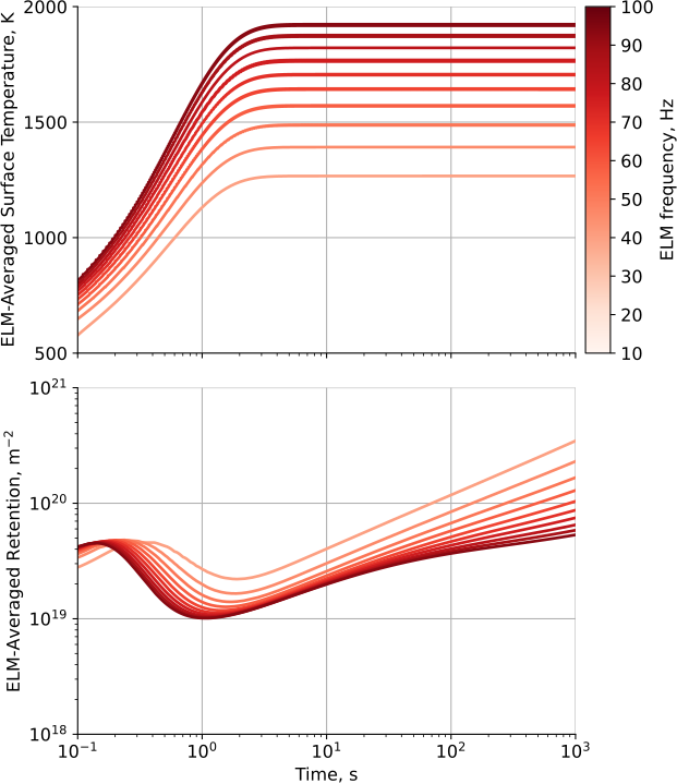
  • 1D model of a ITER monoblock
     
  • Transient heat transfer simulation
     
  • Varying surface heat flux

Detritiation studies

Breeding Blanket modelling

  • DEMO WCLL
  • Complex 3D geometry
  • Coupled to fluid dynamics
  • Tritium generation in the LiPb volume (computed from OpenMC)

James Dark et al 2021 Nucl. Fusion 61 116076

Gas driven permeation

J_\mathrm{left} = K_d \ P - K_r \ c^2
J_\mathrm{right} = - K_r \ c^2

Surface limited regime

Bulk limited regime

Transition to bulk limited as the permeation number \( W \) increases

High H pressure

Low H pressure

Permeation flux

Permeation experiment

No barrier

with barrier

Permeation barrier

Substrate

High H pressure

Low H pressure

Conservation of chemical potential

Permeation flux

\frac{c^-}{K_S^-} = \frac{c^+}{K_S^+}

TDS analysis: neutron damage

\frac{d n}{dt} = \Phi \ K \ (1 - \frac{n}{n_\mathrm{max}}) - A \ n
  • New proposed model for neutron-induced trap creation
     
  • Parameterised on TDS data (self-damaged W)

TDS analysis: codeposits

  • Simulation of W codeposited layers
     
  • Influence of partial pressure
     
  • 10 different traps!

Kinetic surface model

Kinetic surface model

  • D in damaged W (S. Markelj JNM 2016)
     
  • Comparison with NRA (Nuclear Reaction Analysis) profiles

Kinetic surface model

  • H in oxidised W (A. Dunand et al 2022 Nucl. Fusion)
     
  • Comparison with TDS spectra

Kinetic surface model

  • H in Ti (Hirooka et al 1981 JNM)
     
  • Validation at 5 temperatures

H content (H/Ti)

HISP project: coupling FESTIM to plasma codes

RISP pulse

ITER FW divided in 60 bins

Data from DINA

Goal: find the best strategy for minimising ITER T inventory

HISP project: coupling FESTIM to plasma codes

10 DT FP pulses

ICWC + RISP

GDC

Simulation time:
~ 60 s per bin (~ hour full reactor)

Demo: how to install FESTIM

Demo: how to run a python script

FESTIM tutorials

  • Simple simulation
  • TDS simulation
  • Simple permeation simulation
  • Visualisation and post-processing
  • Radioactive decay

UKAEA FESTIM workshop 2026 materials

By Remi Delaporte-Mathurin
UKAEA FESTIM workshop 2026 materials

  • 84