Robert Salomone

Centre for Data Science, Queensland University of Technology (QUT)

Computational Methodology in Statistics and Machine Learning: An Invitation 

Research Elevator Uber Pitch

My response has converged to...

"I use mathematical ideas in creative ways to help improve methods in statistics and machine learning. A large part of this is making computers work more reliably and efficiently for very difficult problems." 

What this talk is about...

• That was the very big picture, this talk is a (slightly) smaller picture - overview of my research contributions.

• Top 5:  Each paper, small amount of background, followed by discussion of things accomplished.

• Recurring Theme: Insights and ideas from diverse areas (maths, statistics, machine learning) help solve problems and develop new methodology. 

• Discussion of some other areas where similar ideas pop up. 

• My Goal (research dissemination aside): Inspire you to think a little about how your insights from different fields may be useful.

• A canonical problem in the computational sciences, statistics, and machine learning is the evaluation of \[\pi(\varphi) := \int \varphi\, {\rm d}\pi.\]
• Most general approach: replace \(\mu\) with some \(\nu^N \), and use

\[\nu^N(\varphi) := \sum_{k=1}^N W_k \varphi(x_k).\]​

• Everything today is based on this idea - how to construct \(\nu^N\) to overcome specific challenges. \[ \] \[ \]

• Popular Approach: The Monte Carlo method. Draw \(N\) samples \(\{ \mathbf{X}_k\}_{k=1}^N\) according to \(\pi\) and set

\[\nu^N(\varphi) = \frac{1}{N}\sum_{k=1}^N \varphi(X_k). \]

• Two issues that occur with the above in difficult problems:
  • Sampling from \(\pi\) directly is not possible / prohibitively expensive
  • The estimator \(\nu^N(\varphi)\) exhibits very high variance

• Such difficult integration problems arise in many settings,  but none so notorious as Bayesian Inference: \[p(\boldsymbol{\theta}| \mathbf{y}) = \frac{p(\boldsymbol{\theta})p(\mathbf{y}|\boldsymbol{\theta})}{\mathcal{Z}}.\]
• The normalizing constant (model evidence aka marginal likelihood) is also of interest: \[\mathcal{Z} = p(\mathbf{y}) = \int p(\boldsymbol{\theta})p(\mathbf{y}|\boldsymbol{\theta}){\rm d}\boldsymbol{\theta} =  \mathbb{E}_{p(\boldsymbol{\theta})}\big[p(\mathbf{y}|\mathbf{\boldsymbol{\theta}})\big] .\]

Challenges

Research Highlights

Paper #1: Background

• (Markov Chain Monte Carlo) Simulate an ergodic Markov Chain \(\{\mathbf{X}_t\}_{t=0}^N\) with stationary distribution \(\pi\). Take iterates after some burn-in period of length \(b\) that ensures the chain is sufficiently close to stationarity,  \[ \]

\[\nu^N(\varphi) = \frac{1}{N-b}\sum_{k=b}^N \varphi(X_k).\]

• Many ways to do this, e.g., Metropolis-Hastings.

• Generally, a computationally expensive approach.

•  
• ​Problem: The really "tough" models do not have this sum decomposition property (i.e., data are dependent).

Salomone R., Quiroz, M., Kohn, R., Villani, M., and Tran, M.N., (2020),

Spectral Subsampling MCMC for Stationary Time Series.

(Contribution) Extending Bayesian methods for large datasets to stationary time series.  

• We take an approach common in statistics: "If data doesn't satisfy a model assumption, transform it so that it does."
  • Elusive solution: Discrete Fourier transform data, obtain periodogram, and use a Frequency Domain likelihood.
    • Works on many models (including Stochastic Volatility)\[ \] 
  • Transformed data are asymptotically independent with known distribution (exponential). \[ \] 
  • Likelihood is in terms of spectral density (Fourier dual of autocovariance function). \[ \] 
  • Close to 100x computational speed-up in examples considered (compared to full data MCMC). 

Paper # 1:

Published in International Conference in Machine Learning (ICML), (2020)

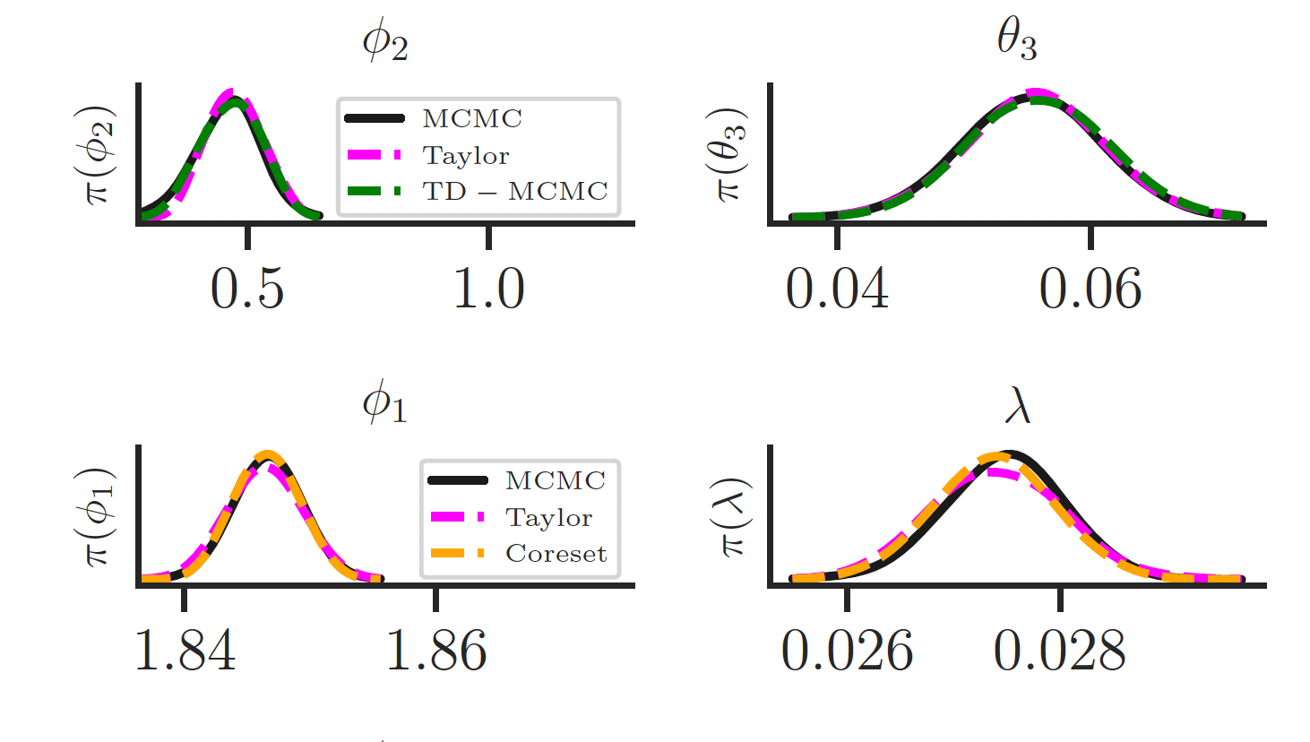
Villani, M., Quiroz, M., Kohn, R., and Salomone, R. (2021), Spectral Subsampling MCMC for Stationary Multivariate Time Series.

Encore (Follow-up Paper)

• (Main Contribution): Extends the approach to vector-valued stationary time series. \[ \]
  • Asymptotic distribution of transformed data now Complex Wishart (Likelihood involves spectral density matrices). \[ \] 
• (Additional Contribution): Introduce a new multivariate time series model (VARTFIMA) involving Tempered Fractional Differencing (TFI), and derive its properties.  \[ \] 
• Even on tough examples, still around 100x computational speed up, again with minimal difference in inferences.

Recently Submitted (Invited Paper)

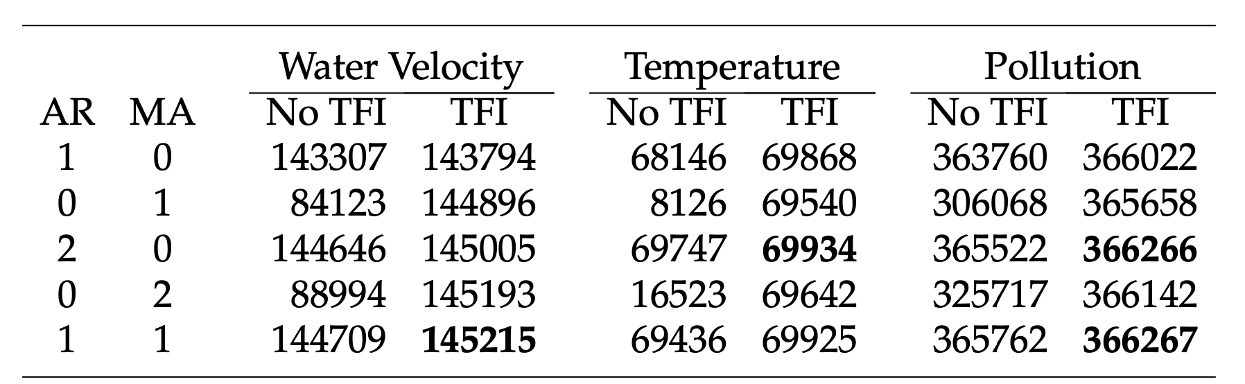
(TFI does very well in terms of BIC)

Paper #2: Background (Uncorrected Samplers)

• Aside from tall data in Bayesian Inference, another significant challenge inference (and sampling in general) is high-dimensionality. In higher dimensions, MCMC tends to converge slowly.

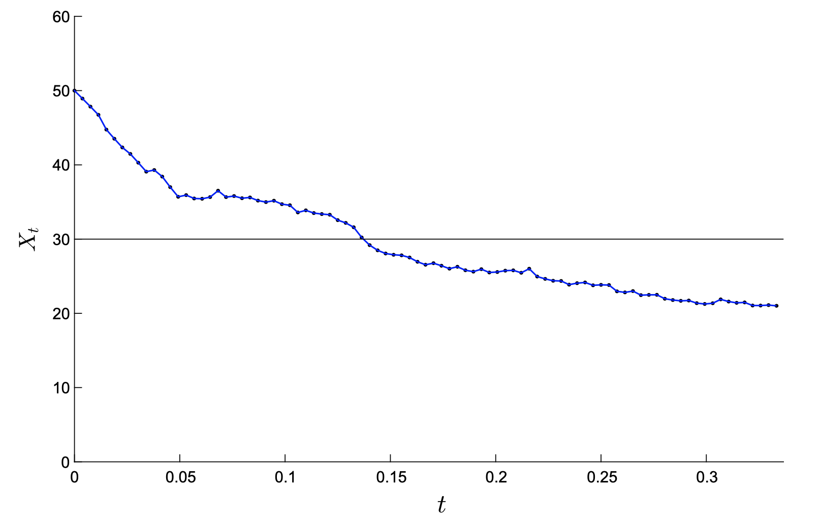
• Langevin Stochastic Differential Equation

\[{\bf X}_0 \sim \nu, \quad {\rm d}{\bf X}_t = \frac{1}{2}\nabla \log \pi({\bf X}_t){\rm d}t + {\rm d}{\bf W}_t, \]

has stationary distribution \(\pi\).

• Euler-Maruyama Approximation of Langevin SDE \[{\bf X}_0 \sim \nu, \quad {\rm d}{\bf X}_t = \frac{1}{2}\nabla \log \pi({\bf X}_t){\rm d}t + {\rm d}{\bf W}_t, \]

has stationary distribution \(\nu \ne \pi\) (or none at all!).

​

• Even when that is not the case, there is still interest in forgoing "asymptotic exactness" for good results in reasonable (finite) time. That is, lower MSE approaches.

A Story...

Hodgkinson, L., Salomone,R., and Roosta, F. (2019),  Implicit Langevin Algorithms for Sampling From Log-concave Densities.

Hodgkinson, L., Salomone,R., and Roosta, F. (2019),  Implicit Langevin Algorithms for Sampling From Log-concave Densities.

Accepted at Journal of Machine Learning Research

#2

Contributions

• Links to Convex Optimization
• Explicit Transition Kernel
• Geometric Ergodicity 
• 2-Wasserstein Bounds (w/ Inexact Solutions)
• CLT for \(h \rightarrow \infty \) (Stability)
• (Pilot-Free) Step Size Heuristic

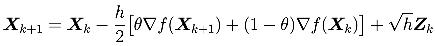
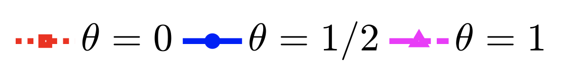
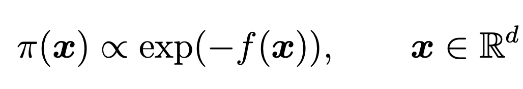
Implicit Discretization of \(\pi\)-ergodic Langevin SDE: 

Unadjusted Algorithm (Asymptotically Biased)

Next Up: Estimating \(\mathcal{Z}\) and sampling from pathologically shaped distributions.

• Nested Sampling (Skilling, 2006) is a method for model evidence and sampling.
  • Very popular in some fields (Astronomy, Physics) but a very unusual method!

\(\pi(\mathbf{x}) = \eta(\mathbf{x}){\mathcal{L}(\mathbf{x}})/{\mathcal{Z}} \)

\(\mathcal{Z} = \mathbb{E}_{\eta}{\mathcal L}(\mathbf{X})  = \int_0^\infty \mathbb{P}_{\eta}({\mathcal{L}(\mathbf{X}) \ge l}){\rm d}l\)

• Problem: Derivation requires unrealistic assumptions such as particle independence and particles having the exact distribution at each step. 

\(0\)

\(1\)

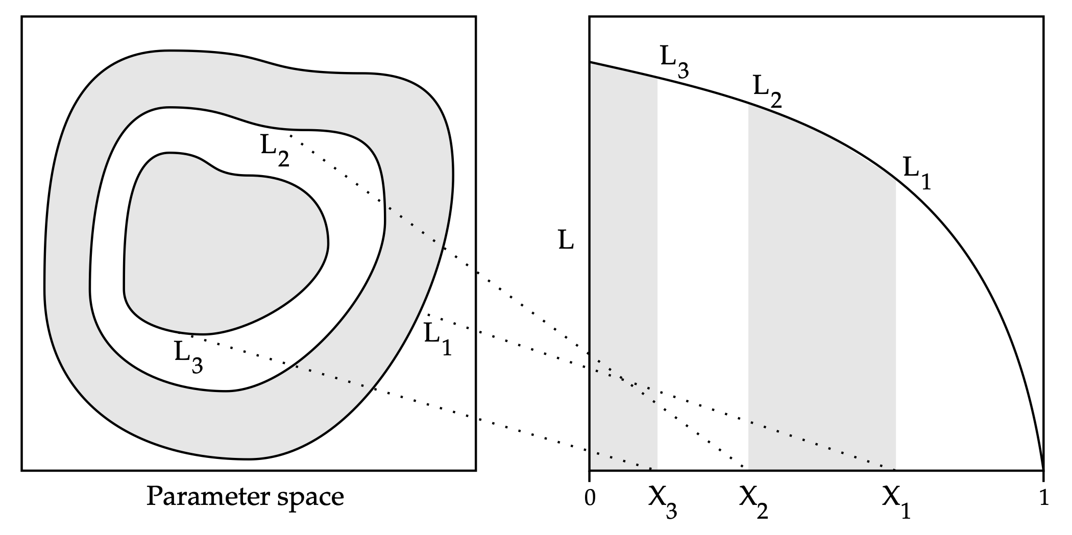
Main Idea: Perform Quadrature to solve...

1. Draw \(X_1, \ldots, X_n \sim_{{\rm iid}} \eta\)

2. Until Termination:

• \(L_t \leftarrow {\rm min}_k {\mathcal{L}(X_k)}\)
• \(k^\star \leftarrow {\rm argmin}_k {\mathcal{L}(X_k)}\),
• Replace \(X_{k^\star} \) with a sample from \(\eta \) conditional on \( \{\mathcal{L} \ge L_t \}\)

Nested Sampling Procedure

Paper # 3: Background (Nested Sampling)

Popular as it can handle many pathological likelihoods and problems (e.g., Potts Model)

• Not just for estimating \(\mathcal{Z} \): \[\pi(\varphi) = \frac{\eta(\varphi \cdot w)}{\eta(w)} \]

where \[w(\mathbf{x}) \propto \frac{\pi(\mathbf{x})}{\eta({\mathbf{x}})} \]

(similar formula to Importance Sampling)

• Useful for Multimodal target distributions.

Paper # 3: Background (Sequential Monte Carlo)

• Importance Sampling Identity: \[\pi(\varphi) = \frac{\eta(\varphi \cdot w)}{\eta(w)} \]

where \[w(\mathbf{x}) \propto \frac{\pi(\mathbf{x})}{\eta({\mathbf{x}})} \]

• Sequential Monte Carlo: Sequential Importance Sampling  with interaction
  • ​Population of \(N\) weighted "particles" \(\{\mathbf{X}_k, w_k \}_{k=1}^N \)

• Resampling, Reweighting, and Moving (MCMC)
• Also provides an estimator of marginal likelihood \(\mathcal{Z}\)
• Also used for multimodal distributions
• Elegant Theory (Feynman-Kac Flows, Interacting Particle Systems )

Suggests using: \[\nu^N(\varphi) := \sum_{k=1}^N W_k \varphi(X_k), \quad \mathbf{X}_k \sim \eta\]​ with

\[W_k = \frac{w(\mathbf{X}_k)}{\sum_{j=1}^N w(\mathbf{X}_j)}\]

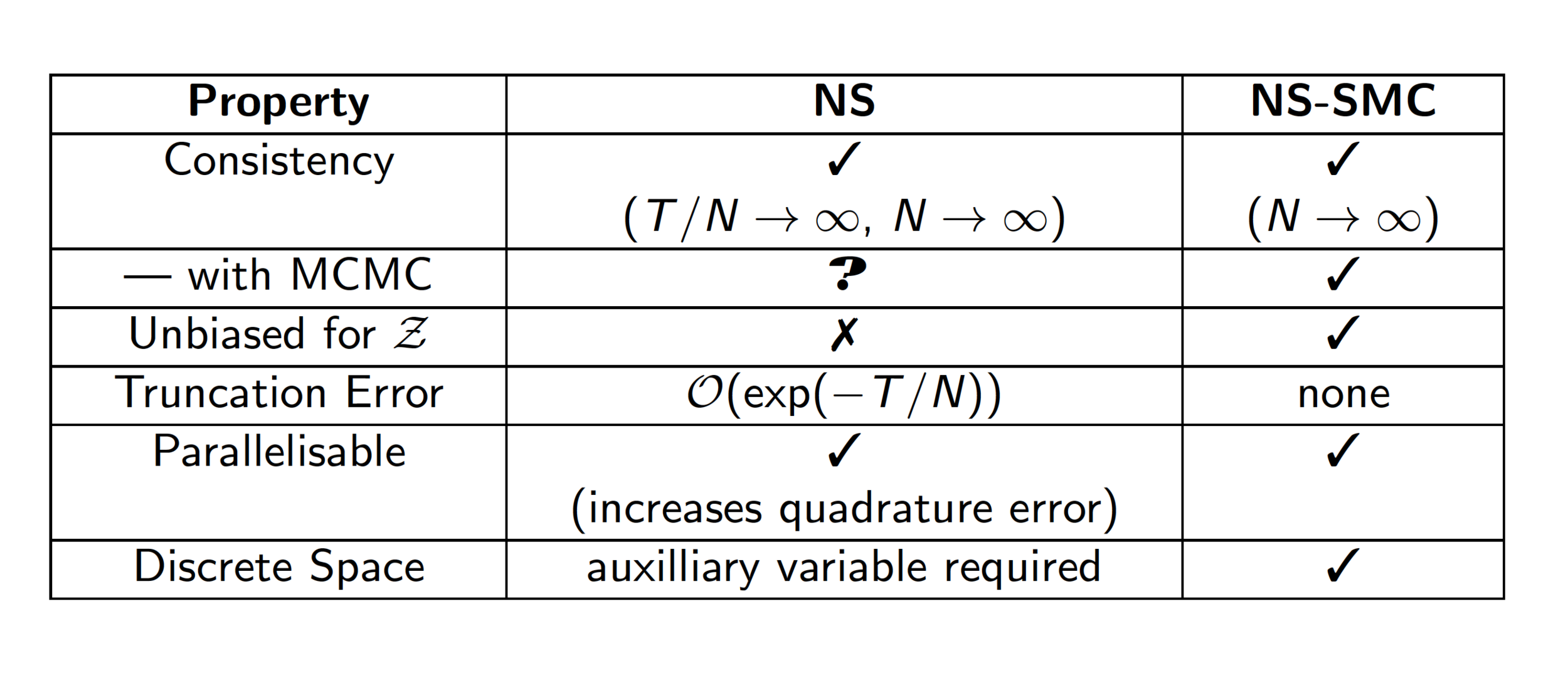
• We establish the link between Nested Sampling and Sequential Monte Carlo
  • ​Nested Sampling is rederived from scratch using Importance Sampling techniques --- whole new class of algorithms!
• Shows how to derive "classic" NS without requiring independence.
• New variants outperform classic NS (optimal estimators fall out of the new derivation).
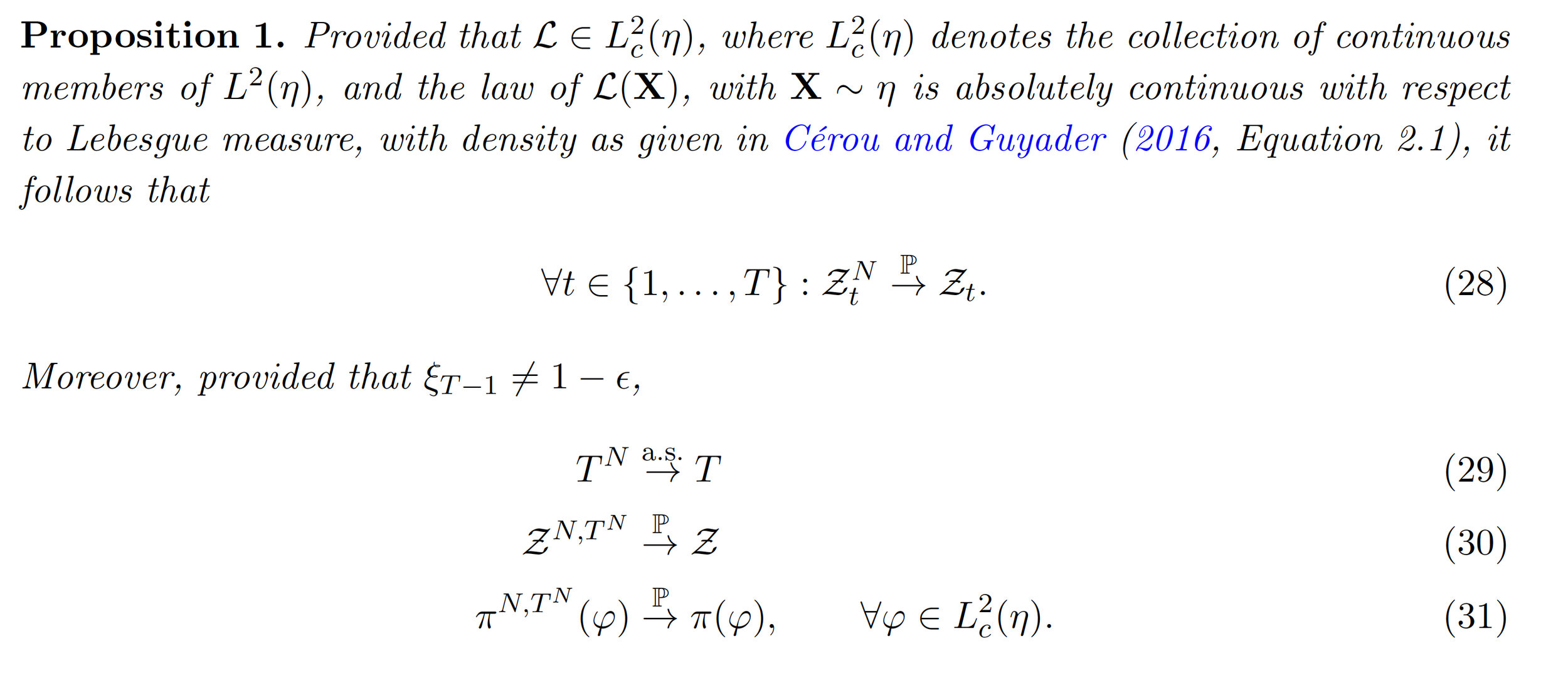
• Theoretical properties are superior (Unbiasedness and Consistency even with dependence!)

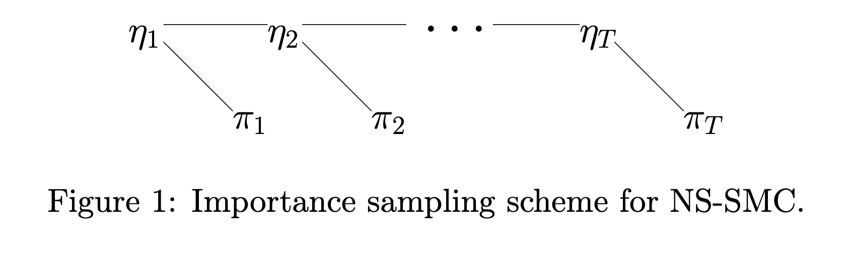
 \(\{\eta_t\} \) : Constrained Priors 

\(\{\pi_t\}\): Constrained Posteriors  

Salomone, R., South, L.F., A.M. Johansen, Drovandi, C.C., and Kroese, D.P.,  Unbiased and Consistent Nested Sampling via Sequential Monte Carlo.

Paper # 3:

Salomone, R., South, L.F., A.M. Johansen, Drovandi, C.C., and Kroese, D.P.,  Unbiased and Consistent Nested Sampling via Sequential Monte Carlo.

Paper # 3:

Long awaited revision almost complete, featuring consistency for the adaptive variant!

Resubmission Pending

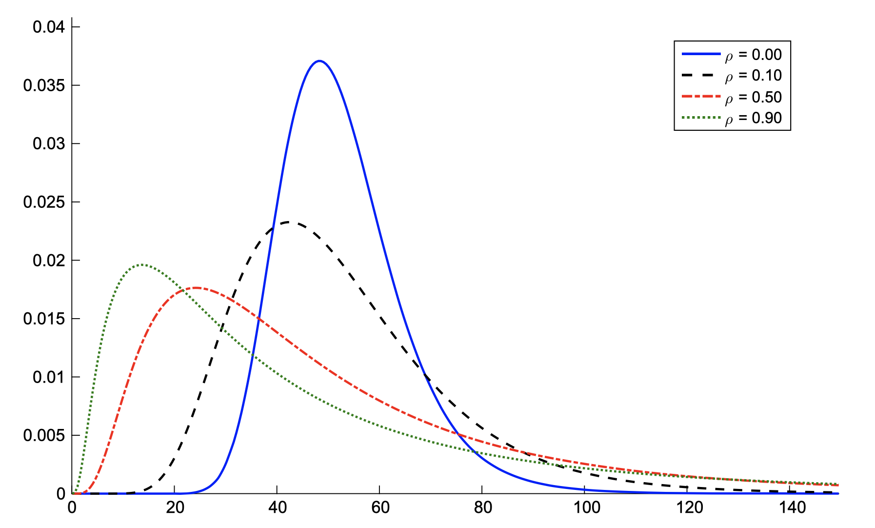
(Dependent) Sum of Lognormals distribution

\(Y = \sum_k \exp(X_k), \quad \mathbf{X} \sim {\mathcal{N}}(\boldsymbol{\mu}, \Sigma). \)

Paper #4: Background (Sum of Lognormals)

• Wireless Communications
• Finance (incl. Black Scholes)

Challenge: Distribution is intractable (even in iid case).

Published in Annals of Operations Research

 Botev, Z.I., Salomone, R., Mackinlay, D., (2019), Fast and accurate computation of the distribution of sums of dependent log-normals.

Contributions

• Efficient estimator of \(\mathbb{P}(Y > \gamma)\) when \(\gamma \rightarrow \infty\)
• Efficient estimator of \(\mathbb{P}(Y < \gamma)\) when \(\gamma\) is very small
• Exact simulation of \(Y | \{Y < \gamma\} \) when \(\gamma \rightarrow 0\)
• Novel estimator for \(f_Y(\cdot)\) 
  • Sensitivity Estimation: \(f_Y(y) = \frac{{\rm d}}{{\rm d}y}\mathbb{P}(Y < y) \)

# 4

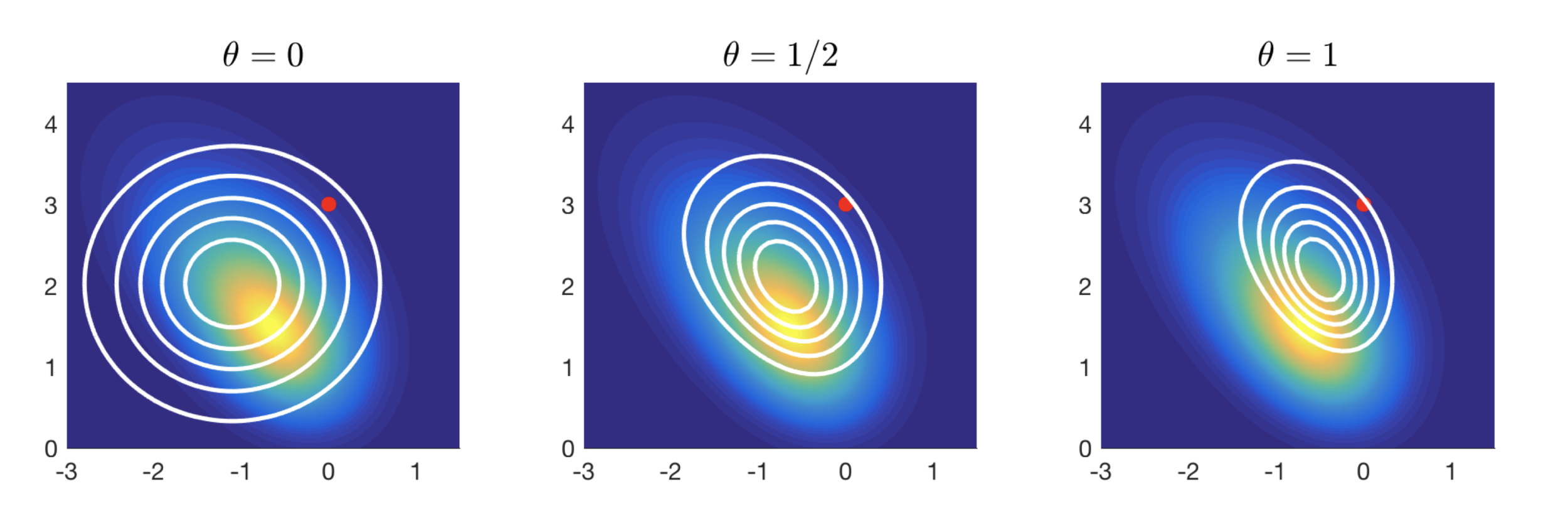
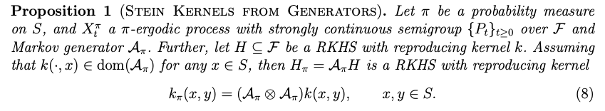
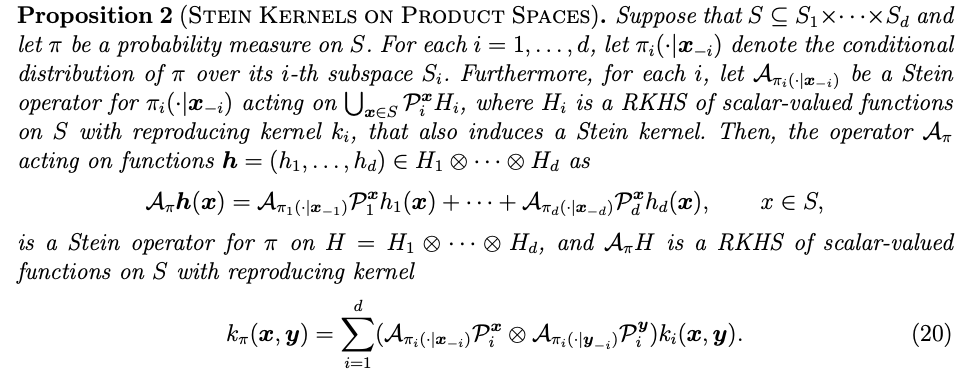
Paper #5: Background (Stein Kernels)

• Key Idea: Stein Operator \(\mathcal{A}_{\pi}\) for \(\pi\) such that for large class of \(\phi \)

​​\[\mathbb{E}\mathcal{A}_\pi \phi(\mathbf{X}) = 0 \Longleftrightarrow  \text{Law}(\mathbf{X})\equiv \pi \]

• Can create a "Steinalized" Kernel \(k_\pi\) - involves essentially applying the Stein Operator to both arguments of some base kernel \(k(\cdot,\cdot) \). \[ \] 
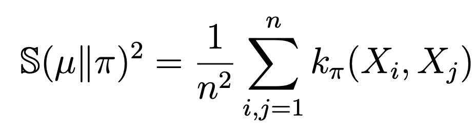
• (Crystal Ball) Kernelized Stein Discrepancy for empirical distributions :

where \(k_\pi\) is a reproducing Stein kernel for \(\pi \), involving terms with \(\nabla \log \pi(\cdot)\).

• \(\mathbb{S}(\mu || \pi) = \sup_{\phi \in \Phi}|\mu(\phi) - \pi(\phi) |\) where \(\Phi\) is the unit ball in a reproducing kernel Hilbert space.

Add kernel methods to the mix...

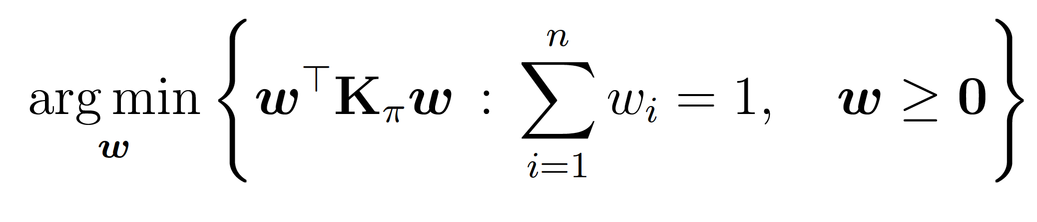
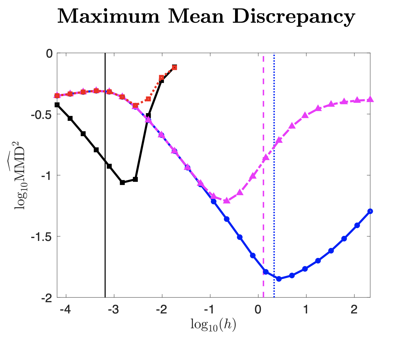
• Stein (Black Box) Importance Sampling Procedure : For fixed samples, assign weights \(w\) that are the solution to

• This is a post-hoc correction (doesn't matter how you get the \(\{X_k\})\).

Hodgkinson, L., Salomone,R., and Roosta, F.,  (2021) The reproducing Stein kernel approach for post-hoc corrected sampling.

A Story...

Hodgkinson, L., Salomone,R., and Roosta, F.,  (2021) The reproducing Stein kernel approach for post-hoc corrected sampling.

(Contributions)

• Method for Construction of KSD on arbitrary Polish spaces. 
  • Based on infinitesimal generator approach.
  • Stein Operator constructed from a stochastic process that has stationary distribution \(\pi\) \[ \] 
• Sufficient conditions for KSD to be separating. \[ \]
  • \(\mathbb{S}(\mu || \pi) = 0 \Longleftrightarrow \mu \equiv \pi \) \[ \] 
• Sufficient conditions for KSD to be convergence-determining on those spaces: \(\mathbb{S}(\nu^n ||\pi) \rightarrow 0 \Longrightarrow \nu^n \stackrel{\mathcal{D}}{\rightarrow} \pi \).

# 5

Distributional Alchemy

• Main Contribution: Convergence of Stein Importance Sampling  for \(\nu\)-ergodic Markov chains.

  • Don't necessarily need \(\nu = \pi\)!

  • Even allows for subsampling!

  • Provides theoretical justification for post-hoc correction of unadjusted samplers.

  • "Best of Both Worlds": Good finite-time behaviour, with good asymptotic properties.

Moral: Ideas are sometimes more connected/useful than one would think.

• Sequential Monte Carlo used to improve Deep Generative Models (e.g., VAE)

• Variance Reduction is used in optimisation algorithms, e.g., stochastic gradient methods.

• Computational tractability is essential in the development of new models and approaches.

Statistics / Machine Learning Research Connection

• Similarly, insights from diverse areas are becoming more important than ever in creating models and algorithms: 
  • Neural ODEs, Differential Geometric Approaches, etc.

Ongoing Work (incl. with Students and Collaborators)

• Variational Inference:   \( \nu^\star = \argmin_{\nu \in \mathcal{Q}}{\mathcal{\mathbb{D}}(\nu || \pi})\)
• Continuous-Time "Non-Reversible"  MCMC (Stochastic Processes)
• Bayesian Experimental Design (Machine Learning)
• Domain-Specific Methodology (Ecology Applications)
• Enhanced SMC (Machine Learning)
• Optimal Transport Approaches (Mathematical Statistics)

Future Interests

• Extensions to existing work (NS-SMC and Stein are particularly promising)
• Focus on intersection of Statistics and ML with more focus on ML.
• Other interesting problems and ideas!

Thanks for listening!