


russtedrake PRO
Roboticist at MIT and TRI
Part II: Sampling-based
MIT 6.800/6.843:
Robotic Manipulation
Fall 2021, Lecture 16
Follow live at https://slides.com/d/wgh6HO0/live
(or later at https://slides.com/russtedrake/fall21-lec16)
subject to:
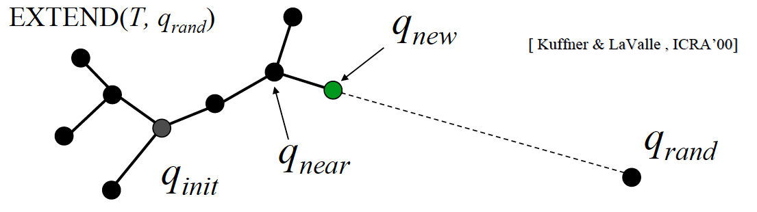
http://www.kuffner.org/james/plan
BUILD_RRT (qinit) {
  T.init(qinit);
  for k = 1 to K do
    qrand = RANDOM_CONFIG();
    EXTEND(T, qrand)
}
http://www.kuffner.org/james/plan
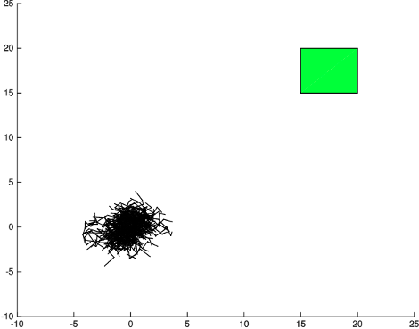
Naive Sampling
RRTs have a "Voronoi-bias"
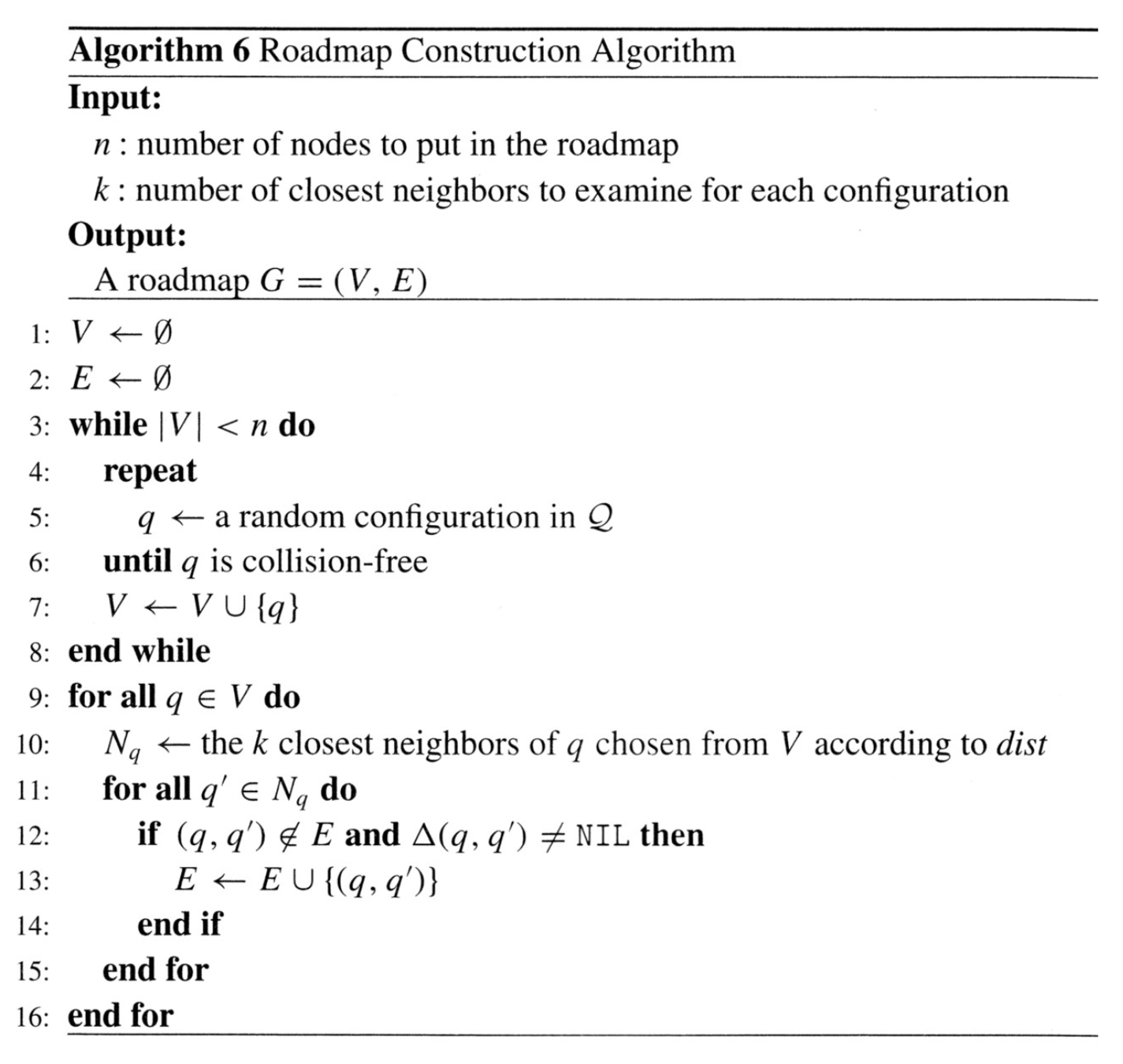
Amato, Nancy M., and Yan Wu. "A randomized roadmap method for path and manipulation planning." Proceedings of IEEE international conference on robotics and automation. Vol. 1. IEEE, 1996.
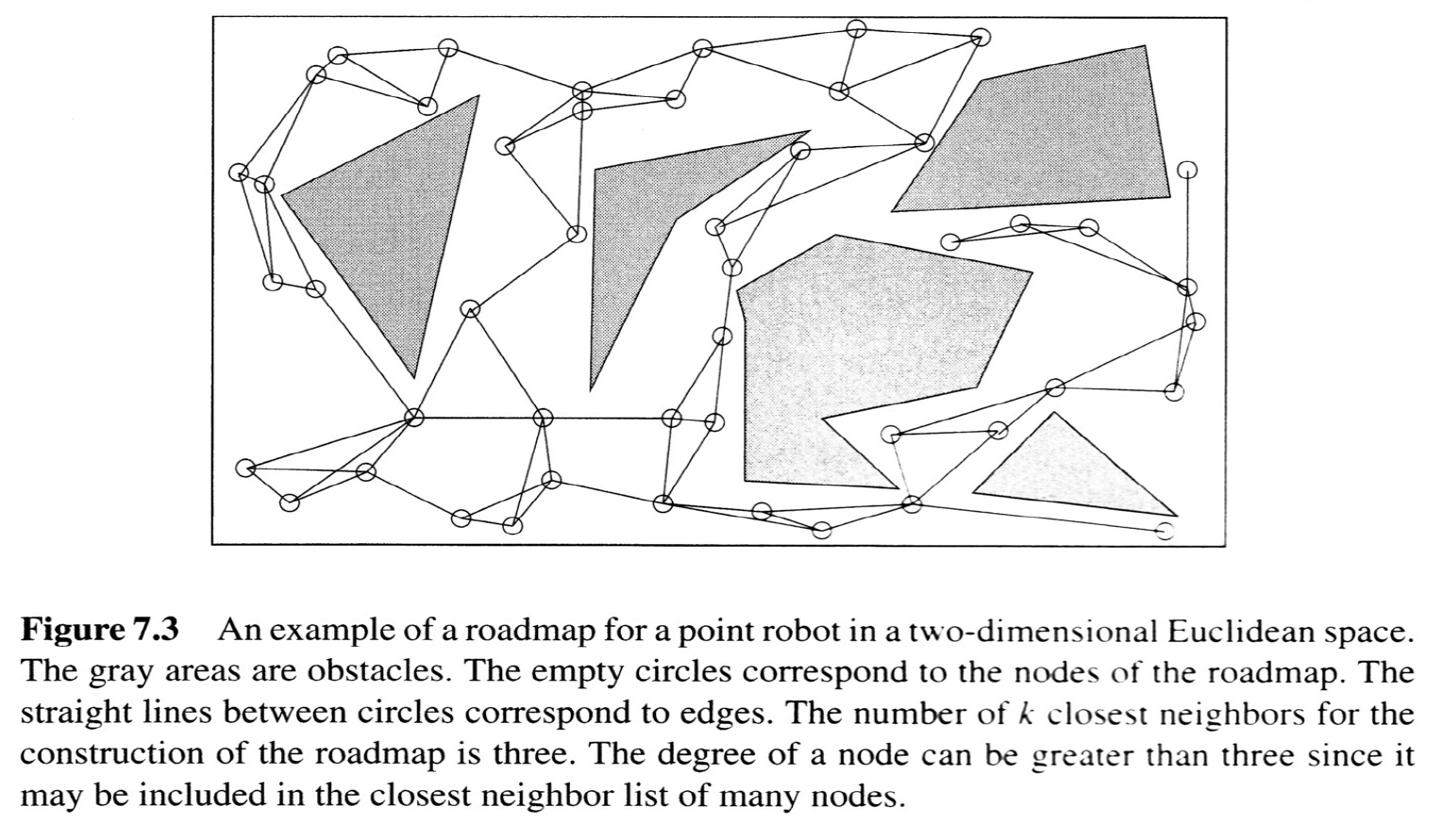
from Choset, Howie M., et al. Principles of robot motion: theory, algorithms, and implementation. MIT press, 2005.
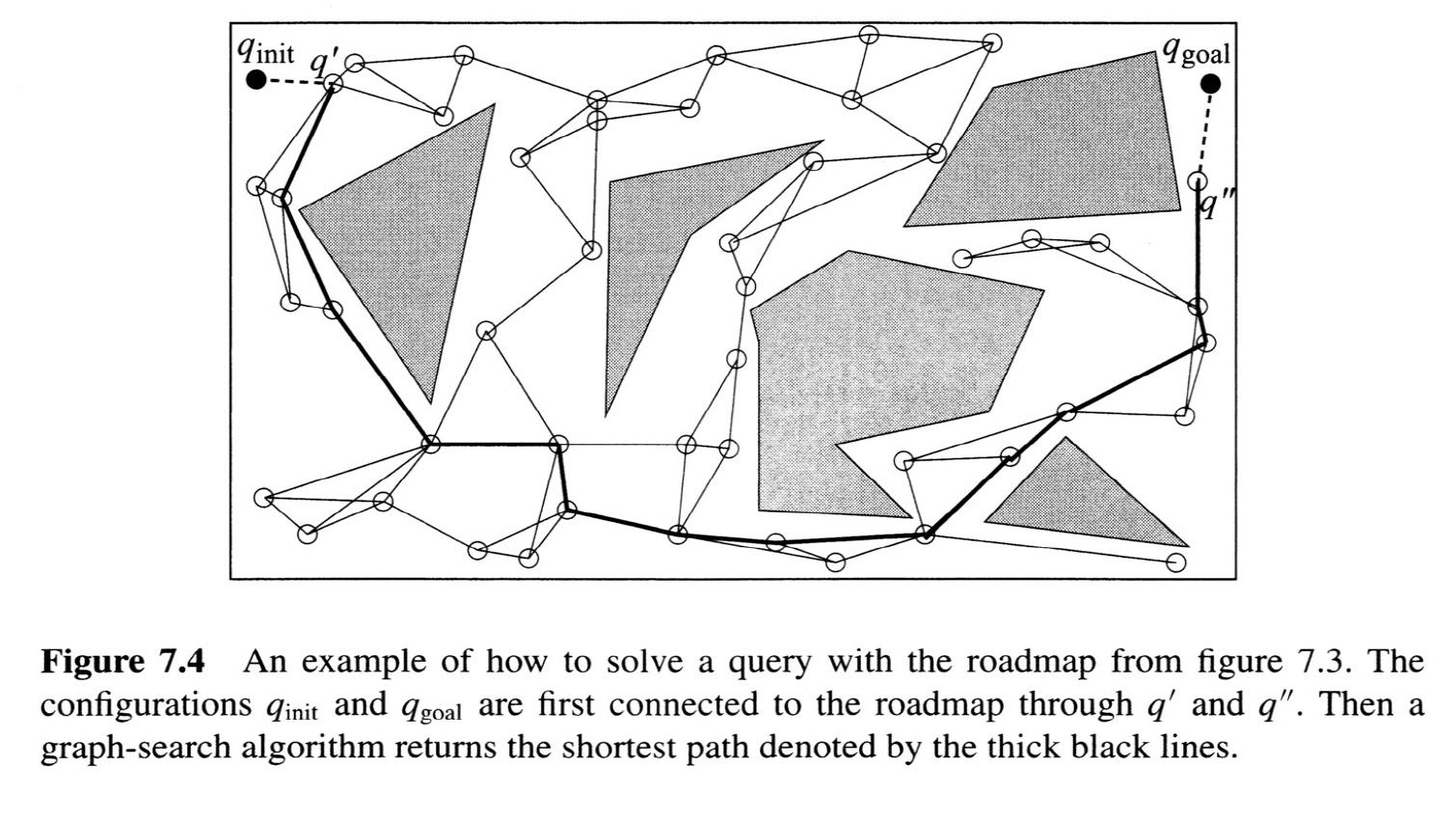
from Choset, Howie M., et al. Principles of robot motion: theory, algorithms, and implementation. MIT press, 2005.
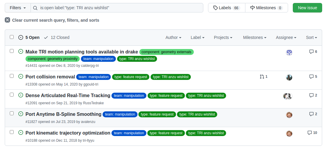
Google "drake+ompl" to find some examples (on stackoverflow) of drake integration in C++. Using the python bindings should work, too.
/**
 * Optimizes the position trajectory of a multibody model. The trajectory is
 * represented as a B-form spline.
 */
class KinematicTrajectoryOptimization {
 public:
  DRAKE_DEFAULT_COPY_AND_MOVE_AND_ASSIGN(KinematicTrajectoryOptimization);

  /// Constructs an optimization problem for a `num_positions`-element position
  /// trajectory represented as a `spline_order`-order B-form spline with
  /// `num_control_points` control_points. The initial guess used in solving the
  /// optimization problem will be the zero-trajectory.
  KinematicTrajectoryOptimization(int num_positions, int num_control_points,
                                  int spline_order = 4);
/// Plans a path using a bidirectional RRT from start to goal.
PlanningResult PlanBiRRTPath(
    const Eigen::VectorXd& start, const Eigen::VectorXd& goal,
    const BiRRTPlannerParameters& parameters,
    const CollisionCheckerBase& collision_checker,
    const std::unordered_set<drake::multibody::BodyIndex>& ignored_bodies,
    StateSamplingInterface<Eigen::VectorXd>* sampler);

/// Bidirectional T-RRT planner.
CostPlanningResult PlanTRRTPath(
    const CostPlanningStateType& start, const Eigen::VectorXd& goal,
    const TRRTPlannerParameters& parameters,
    const CollisionCheckerBase& collision_checker,
    const std::unordered_set<drake::multibody::BodyIndex>& ignored_bodies,
    const MotionCostFunction& motion_cost_function,
    StateSamplingInterface<Eigen::VectorXd>* sampler);


/// Roadmap creation and updating for kinematic PRM planning.

/// Generate a roadmap.
Graph<Eigen::VectorXd> BuildRoadmap(
    int64_t roadmap_size, int64_t num_neighbors,
    const CollisionCheckerBase& collision_checker,
    const std::unordered_set<drake::multibody::BodyIndex>& ignored_bodies,
    StateSamplingInterface<Eigen::VectorXd>* sampler);

/// Plans a path through the provided roadmap. In general, you should use the
/// *AddingNodes versions whenever possible to avoid copies of roadmap.
PlanningResult PlanPRMPath(
    const Eigen::VectorXd& start, const Eigen::VectorXd& goal,
    int64_t num_neighbors, const CollisionCheckerBase& collision_checker,
    const std::unordered_set<drake::multibody::BodyIndex>& ignored_bodies,
    const Graph<Eigen::VectorXd>& roadmap, bool parallelize = true);
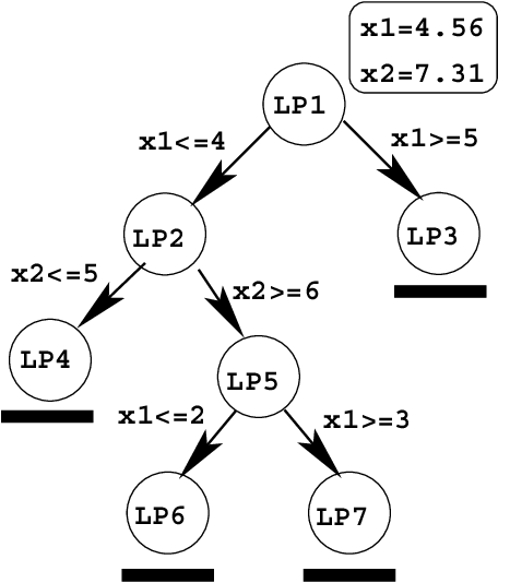
Tobia Marcucci, Jack Umenberger, Pablo Parrilo, Russ Tedrake. Shortest Paths in Graphs of Convex Sets. (Under review)
Available at: https://arxiv.org/abs/2101.11565
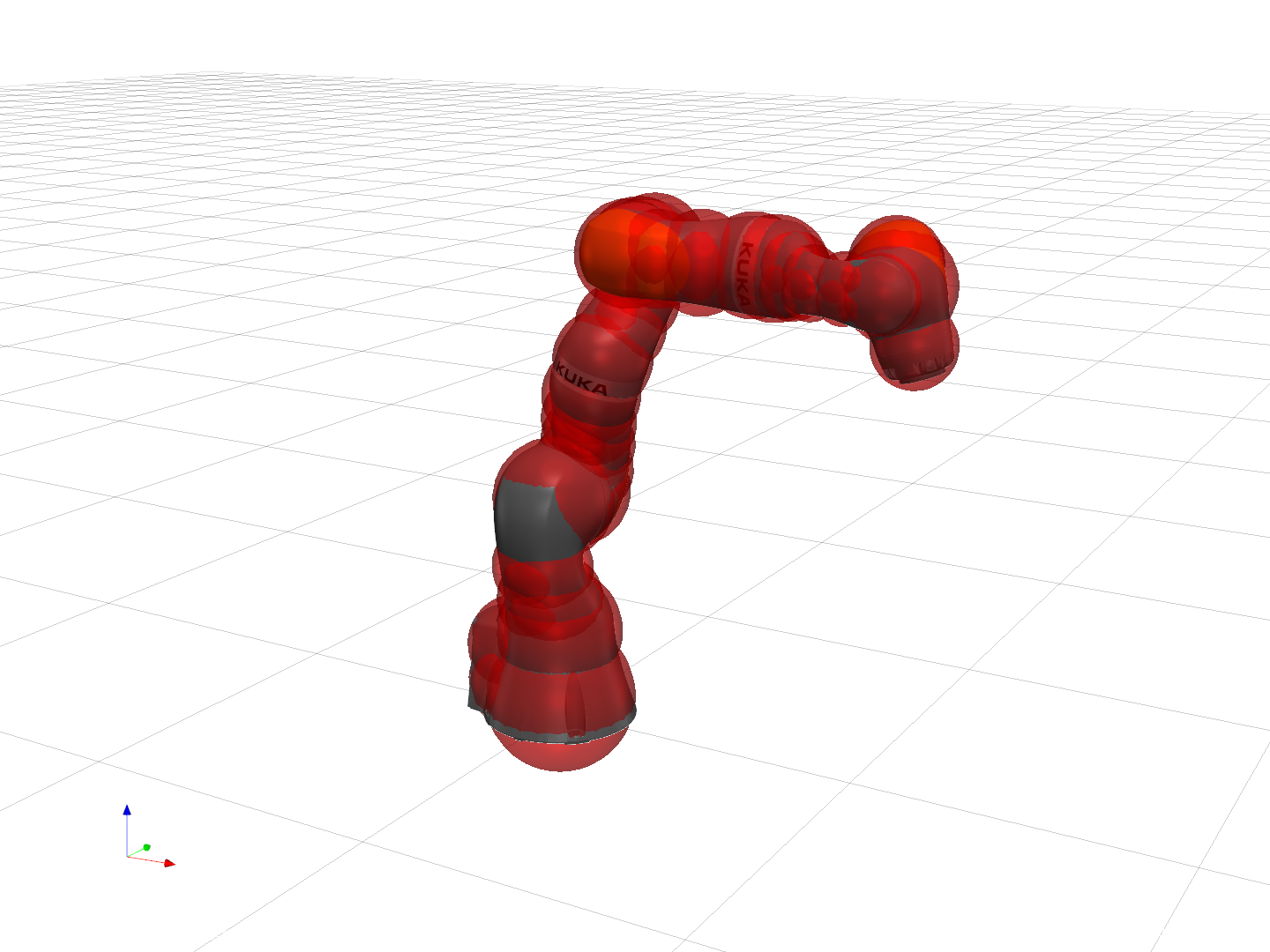
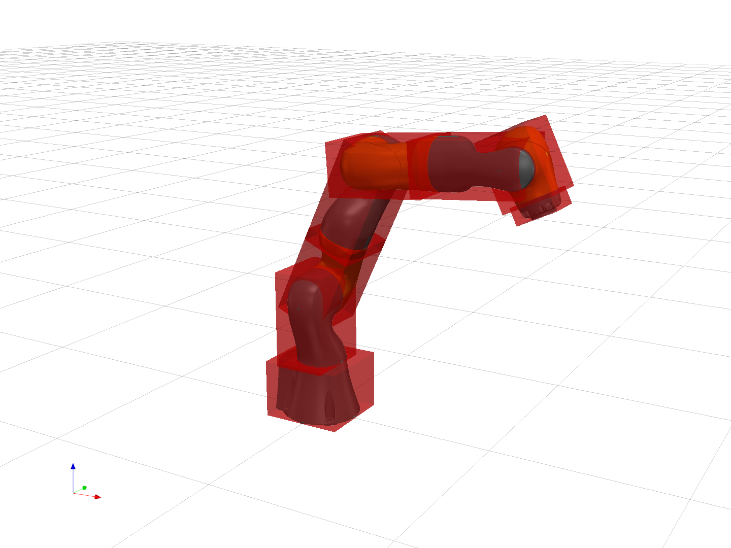
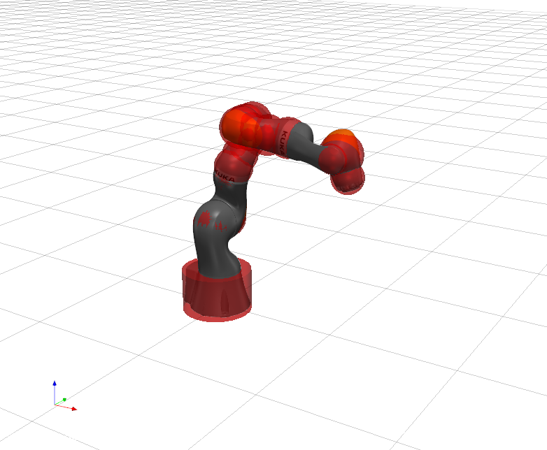
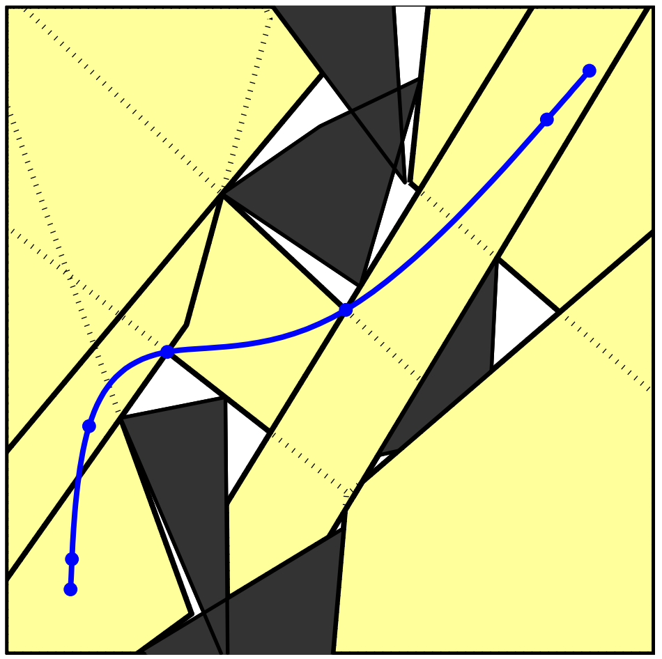
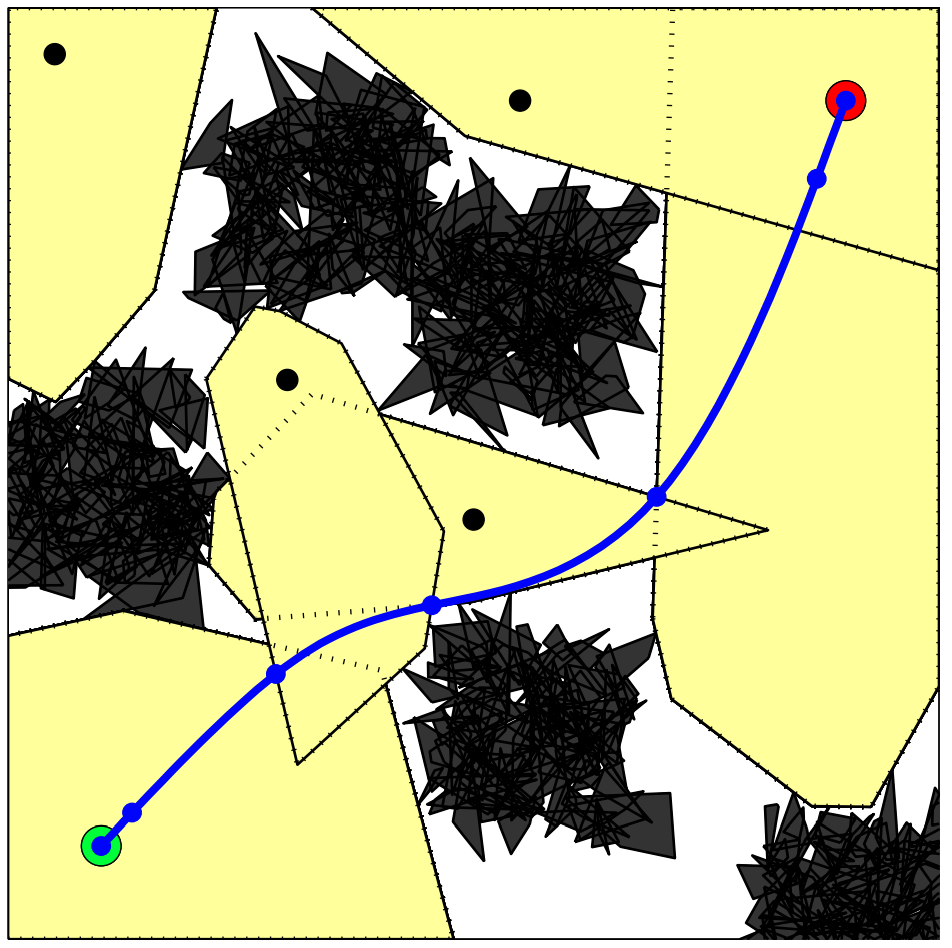
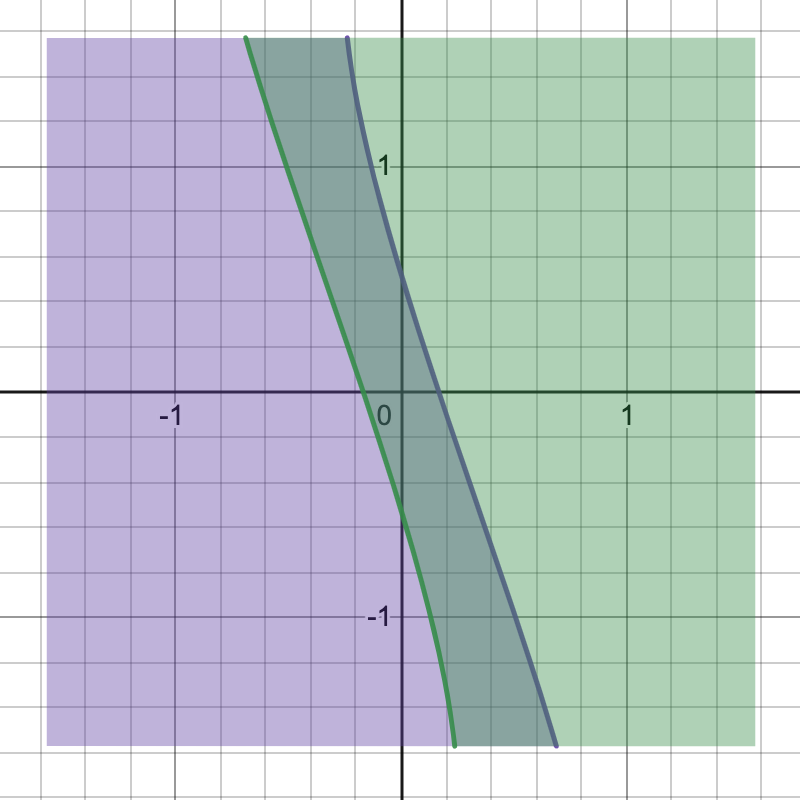
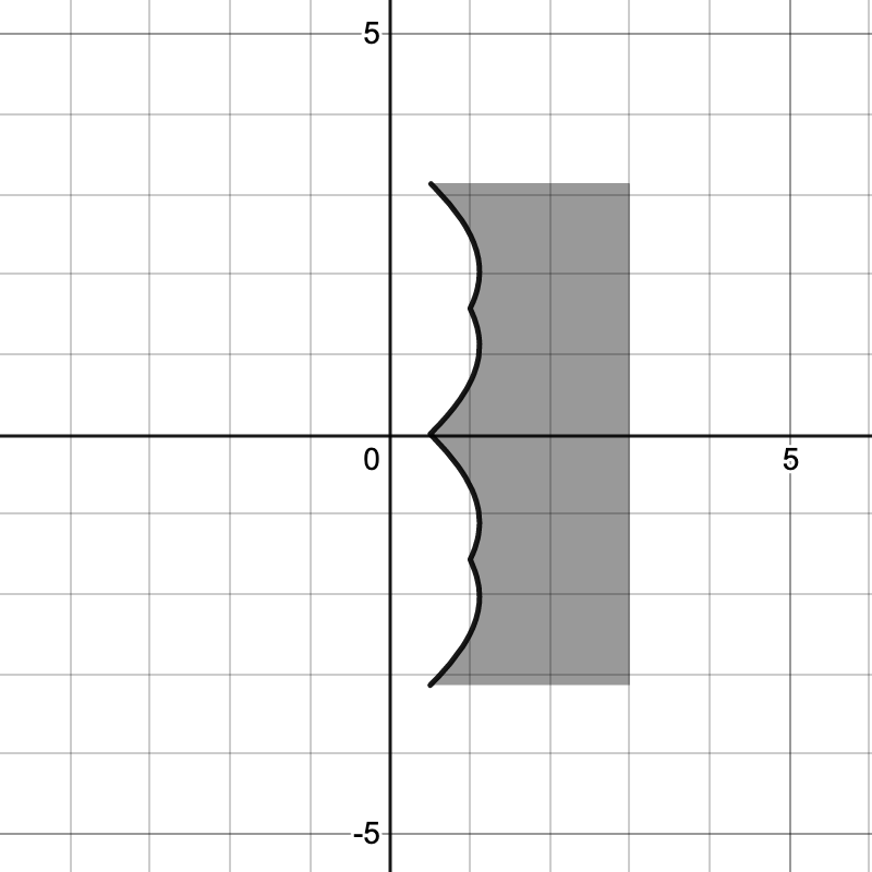
IRIS (Fast approximate convex segmentation)
"We know that the LP formulation of the shortest path problem is tight. Why exactly are your relaxations loose?"
\(\varphi_{ij} = 1\) if the edge \((i,j)\) in shortest path, otherwise \(\varphi_{ij} = 0.\)
\(c_{ij} \) is the (constant) length of edge \((i,j).\)
"flow constraints"
binary relaxation
path length
Classic shortest path LP
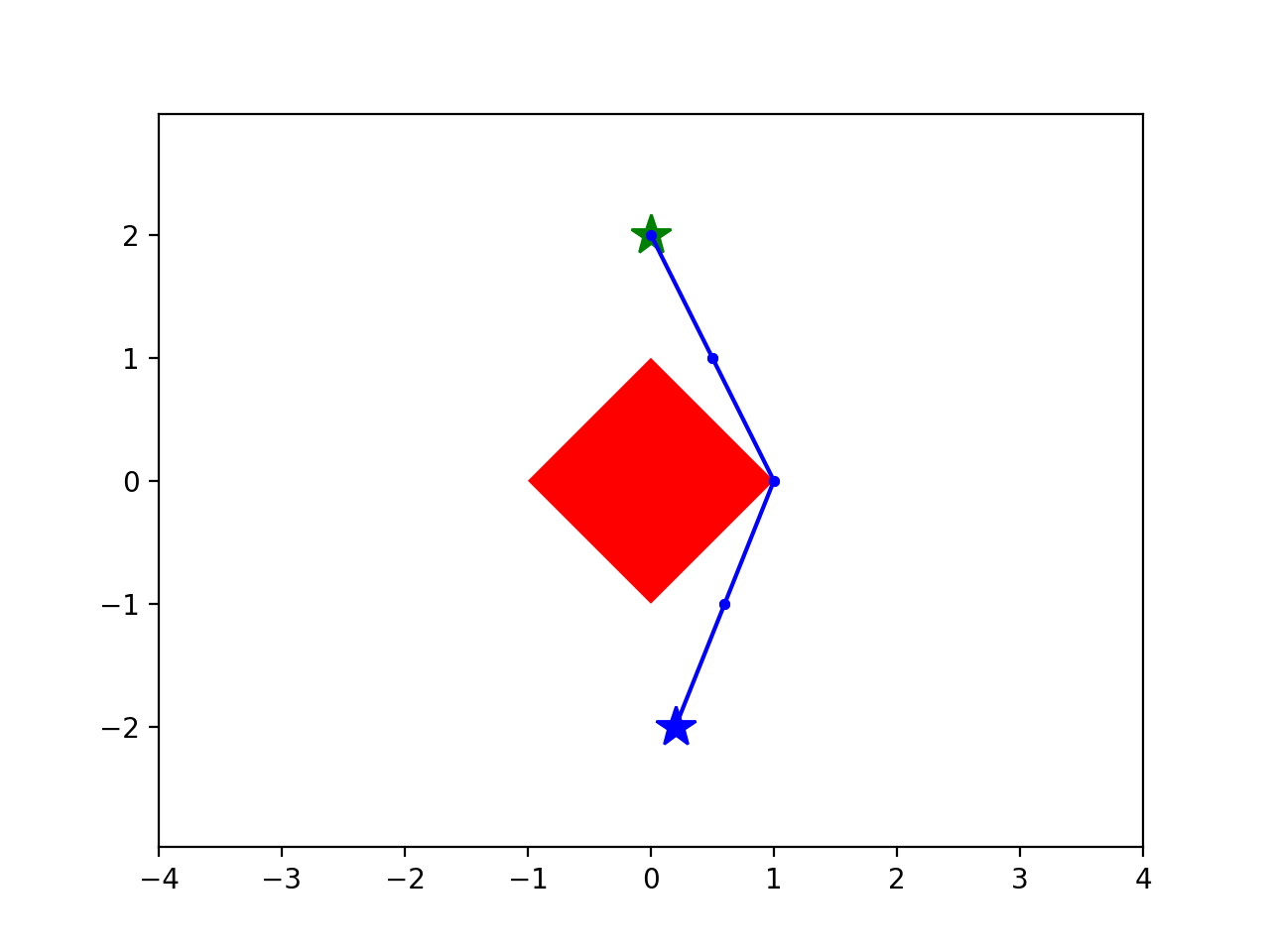
now w/ Convex Sets
start
goal
Step 3:
New formulation
Note: Path length is no longer predetermined
is the convex relaxation. (it's tight!)
| Previous best formulations | New formulation | |
|---|---|---|
| Lower Bound (from convex relaxation) |
7% of MICP | 80% of MICP |
work w/ Andres Valenzuela
work w/ Soonho Kong
work w/ Mark Petersen
Remember: I don't love "collision-free motion planning" as a formulation...
By russtedrake
MIT Robotic Manipulation Fall 2020 http://manipulation.csail.mit.edu


