


russtedrake PRO
Roboticist at MIT and TRI
Russ Tedrake
RSS 2022 Workshop on Differentiable Physics for Robotics
Follow live at https://slides.com/d/PcFMXLM/live
(or later at https://slides.com/russtedrake/rss-differentiable)
Do Differentiable Simulators Give Better Policy Gradients?
H. J. Terry Suh and Max Simchowitz and Kaiqing Zhang and Russ Tedrake
ICML 2022
Available at: https://arxiv.org/abs/2202.00817
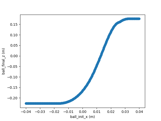
Before we take gradients, let's discuss the optimization landscape...
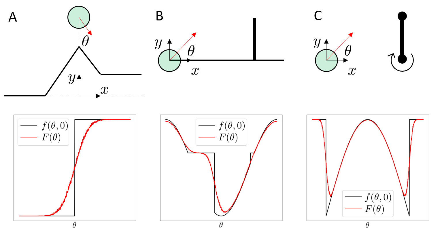
Contact dynamics can lead to discontinuous landscapes, but mostly in the corner cases.
A key question for the success of gradient-based optimization
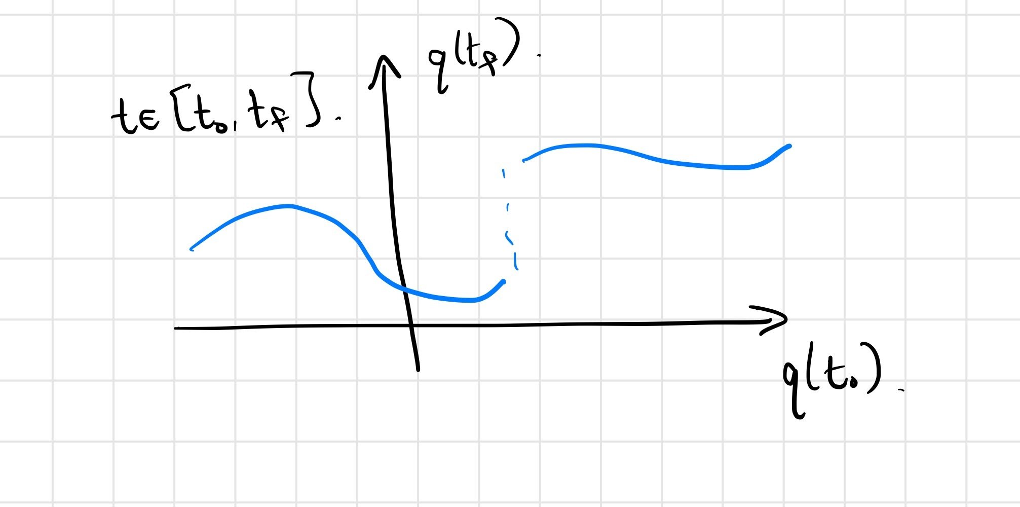
Use initial conditions here as a surrogate for dependence on policy parameters, etc.; final conditions as surrogate for reward.
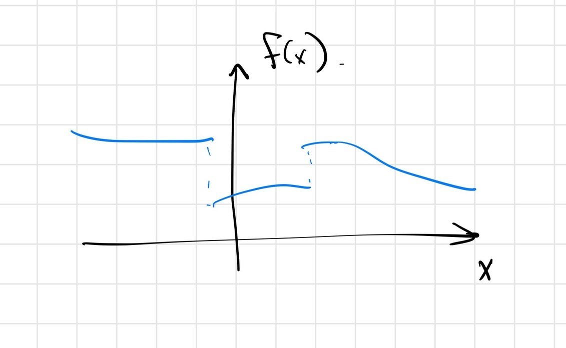
For the mathematical model... (ignoring numerical issues)
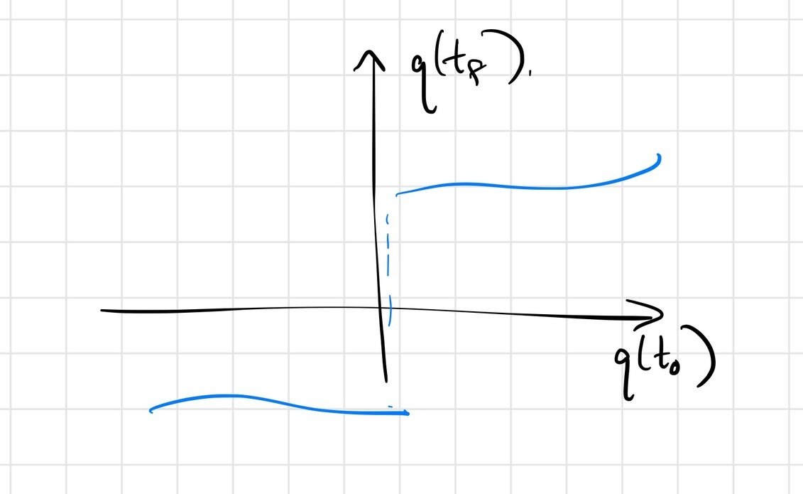
we do expect \(q(t_f) = F\left(q(t_0)\right)\) to be continuous.
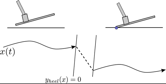
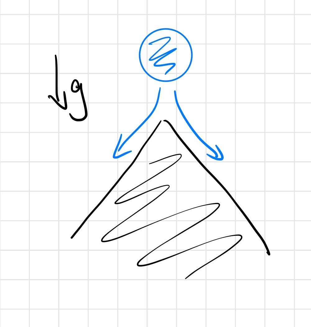
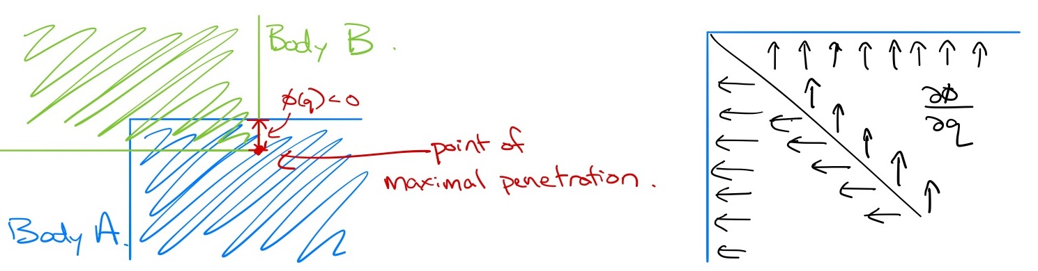
point contact on half-plane
We have "real" discontinuities at the corner cases
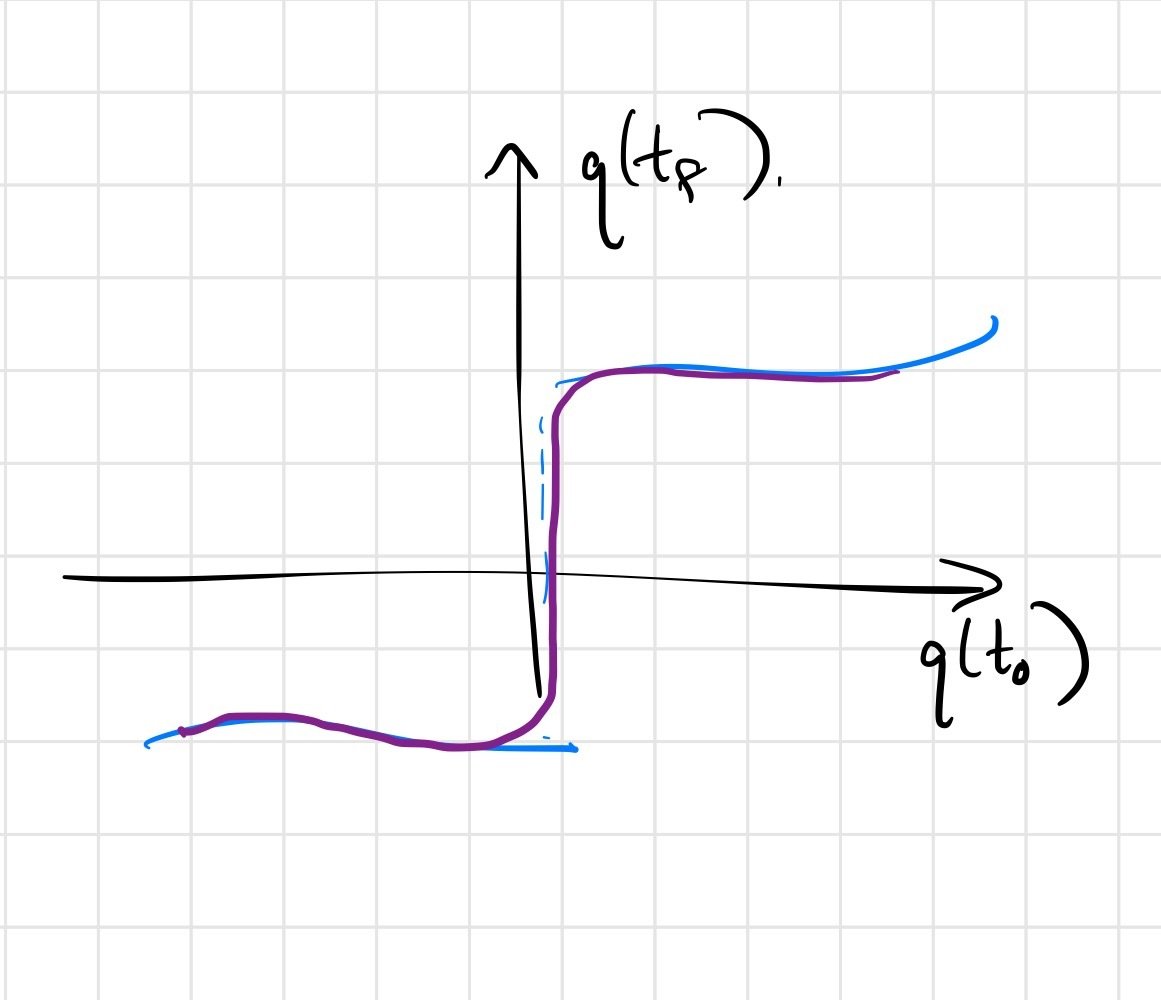
Soft/compliant contact can replace discontinuities with stiff approximations
\[ \min_x f(x) \]
For gradient descent, discontinuities / non-smoothness can
vs
In reinforcement learning (RL) and "deep" model-predictive control, we add stochasticity via
then optimize a stochastic optimal control objective (e.g. maximize expected reward)
These can all smooth the optimization landscape.
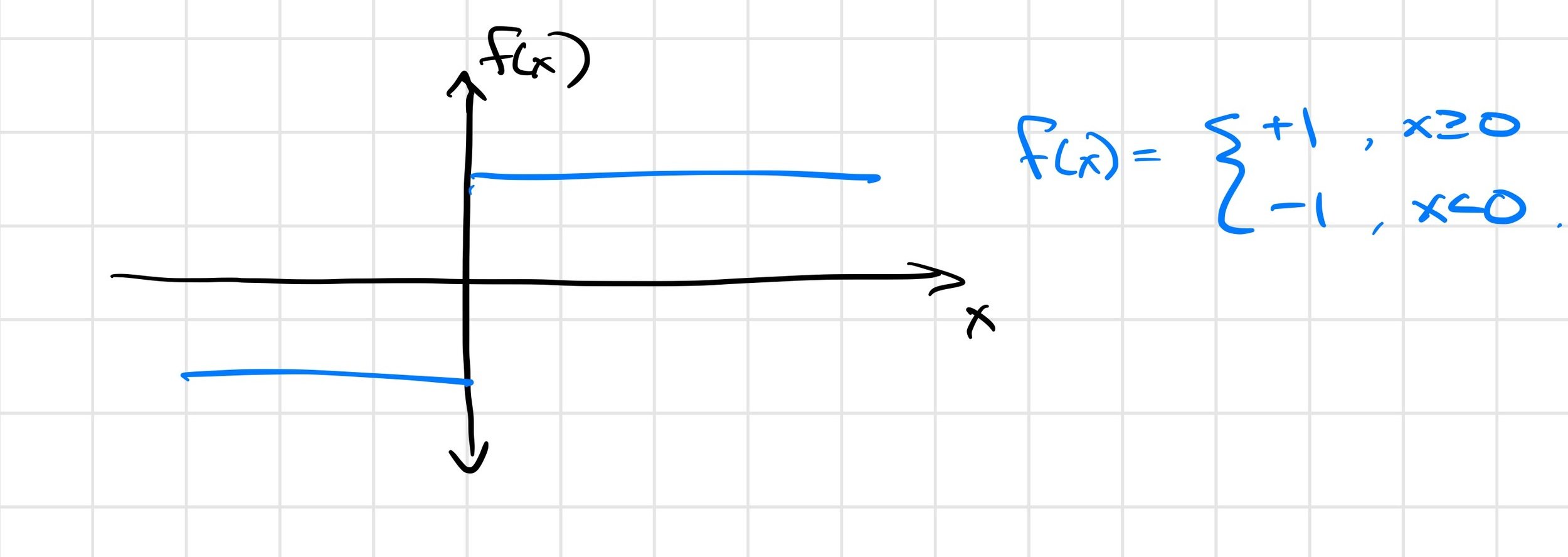
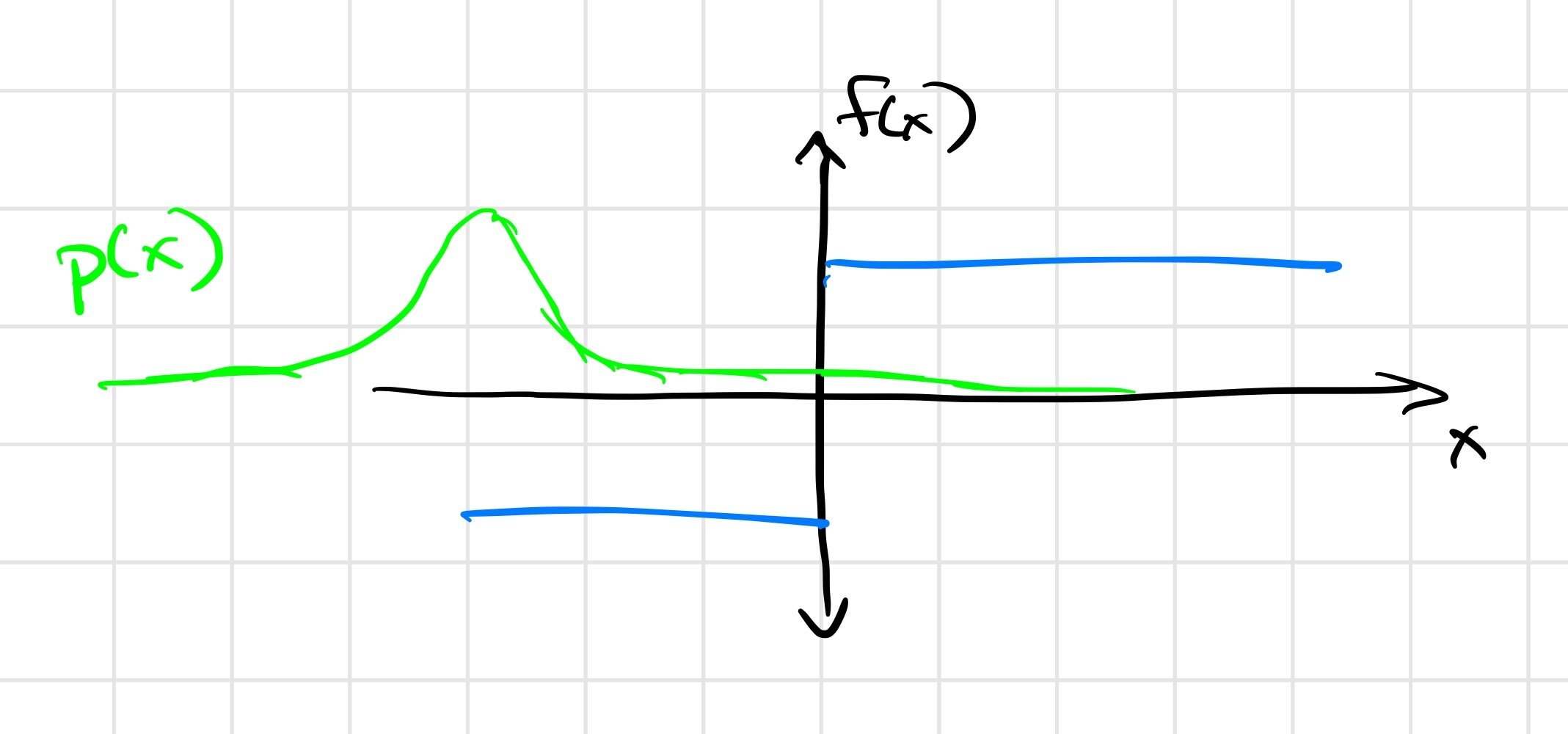
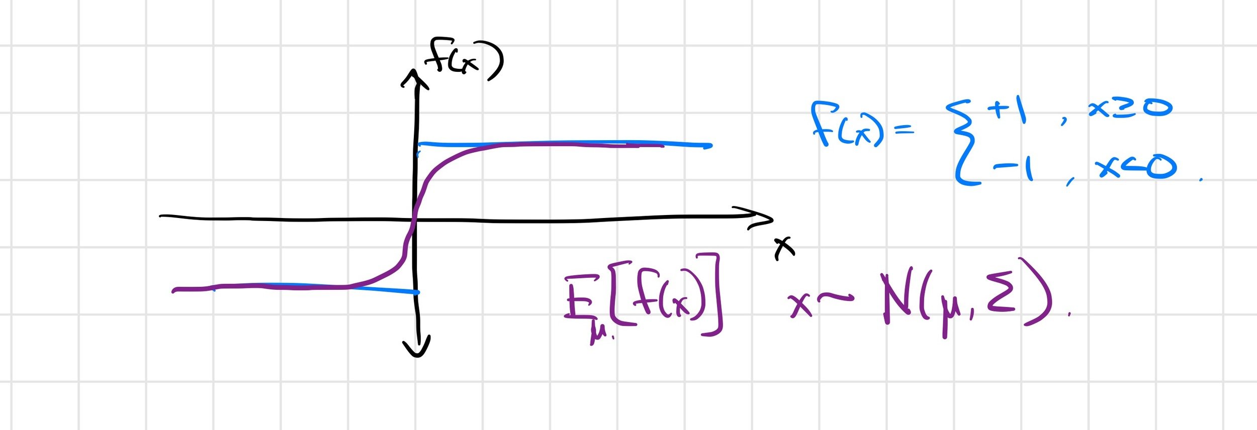
The answer is subtle; the Heaviside example might shed some light.
vs
Differentiable simulators give \(\frac{\partial f}{\partial \theta}\), but we want \(\frac{\partial}{\partial \theta} E_w[f(\theta, w)]\).
J. Burke, F. E. Curtis, A. Lewis, M. Overton, and L. Simoes, Gradient Sampling Methods for Nonsmooth Optimization, 02 2020, pp. 201–225.
But the regularity conditions aren't met in contact discontinuities, leading to a biased first-order estimator.
Often, but not always.
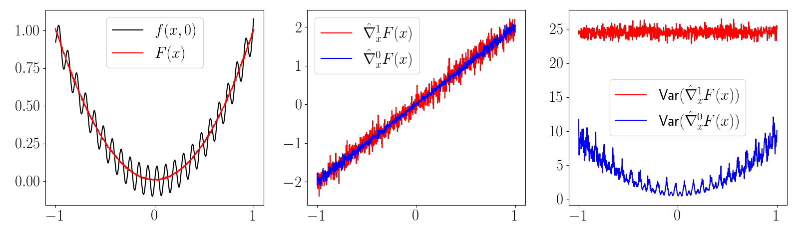
\(\frac{\partial f(x)}{\partial x} = 0\) almost everywhere!
\( \Rightarrow \frac{1}{K} \sum_{i=1}^K \frac{\partial f(\mu + w_i)}{\partial \mu} = 0 \)
First-order estimator is biased
\( \not\approx \frac{\partial}{\partial \mu} E_\mu [f(x)] \)
Zero-order estimator is (still) unbiased
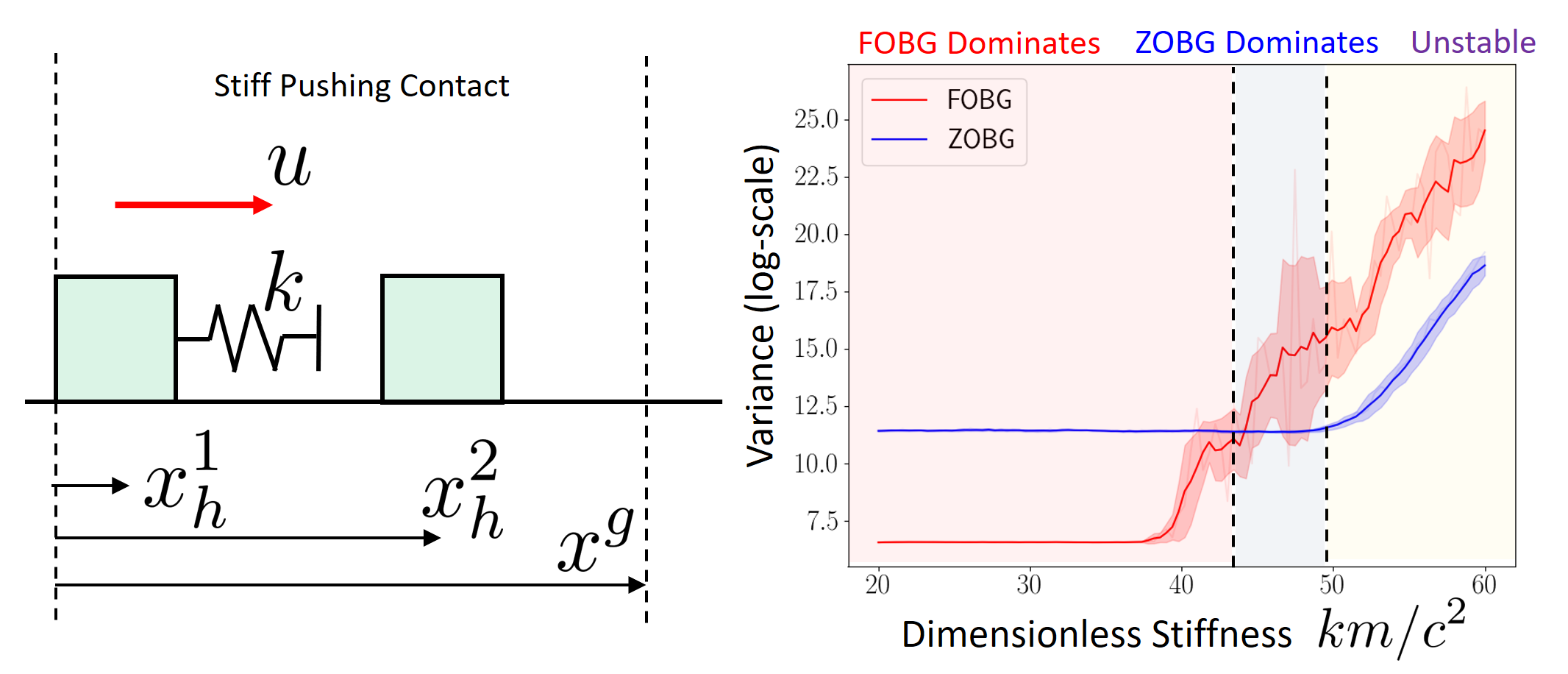
e.g. with stiff contact models (large gradient \(\Rightarrow\) high variance)
First-order estimators are often lower variance that zero-order estimators. But they have some pathologies:
Zero-order estimators are robust in these regimes.
This may explain the experimental success of zero-order methods in contact-rich RL.
Define \(\alpha\)-order gradient estimate as
first-order estimate
zero-order estimate
We give an algorithm to choose \(\alpha\) automatically based on the empirical variance
(+ a trust region using empirical bias).
Smoothing of time-stepping contact model
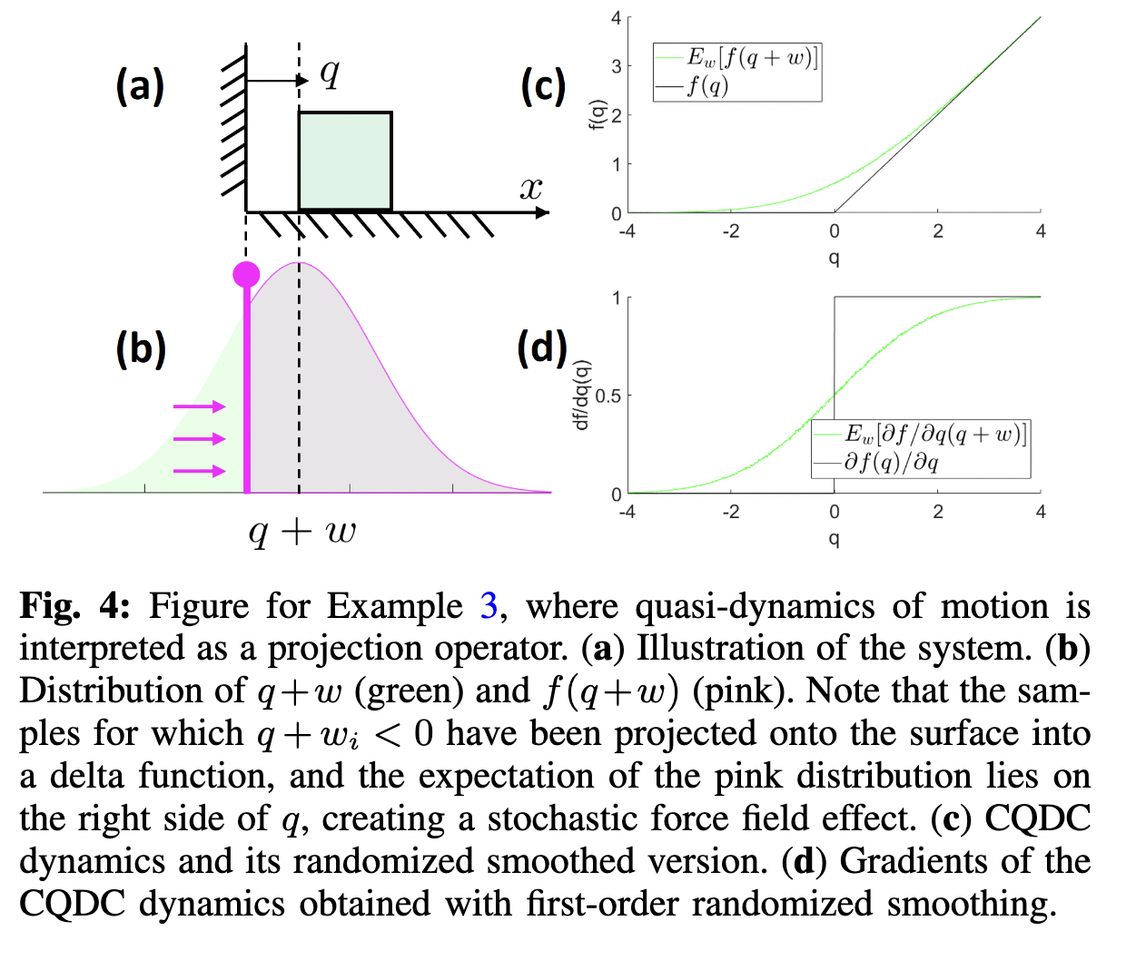
Global Planning for Contact-Rich Manipulation via
Local Smoothing of Quasi-dynamic Contact Models
Tao Pang, H. J. Terry Suh, Lujie Yang, and Russ Tedrake
Available at: https://arxiv.org/abs/2206.10787
Establish equivalence between randomized smoothing and a (deterministic/differentiable) force-at-a-distance contact model.
Gradients
Smoothed gradients (under distribution \(\rho\))
Do Differentiable Simulators Give Better Policy Gradients?
H. J. Terry Suh and Max Simchowitz and Kaiqing Zhang and Russ Tedrake
ICML 2022
Available at: https://arxiv.org/abs/2202.00817
Global Planning for Contact-Rich Manipulation via
Local Smoothing of Quasi-dynamic Contact Models
Tao Pang, H. J. Terry Suh, Lujie Yang, and Russ Tedrake
Available at: https://arxiv.org/abs/2206.10787
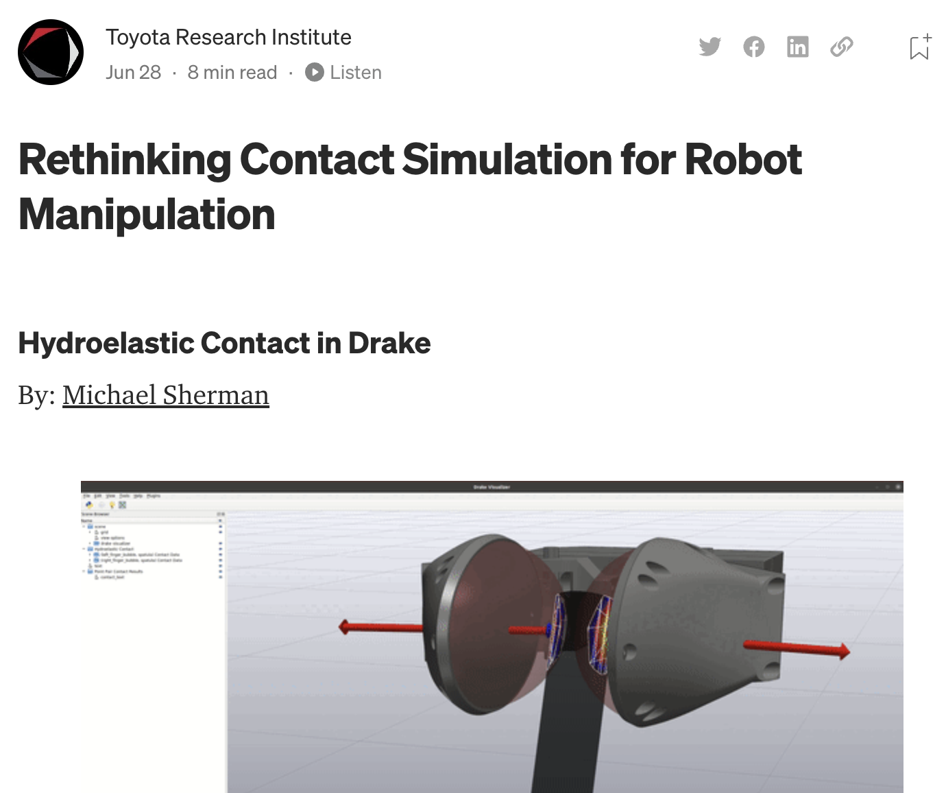
Blog post on "hydroelastic" contact modeling in Drake
Available on Medium.
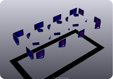
My claim: Subtle interactions between the collision and physics engines can cause artificial discontinuities
(sometimes with dramatic results)
Understanding this requires a few steps
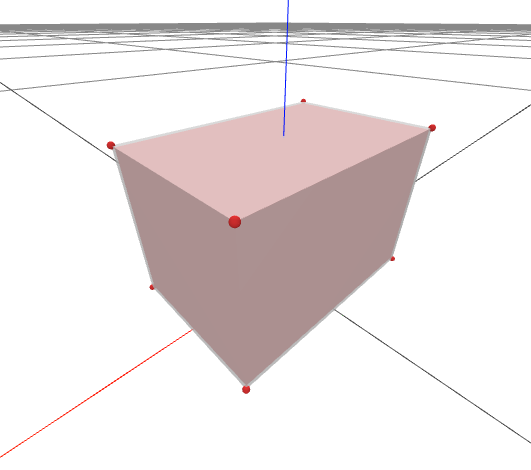
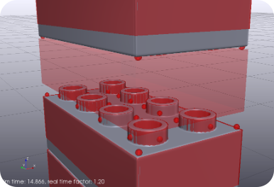
Green arrow is the force on the red box due to the overlap with the blue box.
Many heuristics for using multiple points...
major contributions from Damrong Guoy, Sean Curtis, Rick Cory, Alejandro Castro, ...
Red box is rigid, blue box is soft.
Both boxes are soft.
Point contact (discontinuous)
Hydroelastic
(continuous)
vs
Hydroelastic is
State-space (for simulation, planning, control) is the original rigid-body state.
Point contact and multi-point contact can produce qualitatively wrong behavior.
Hydroelastic often resolves it.
Manually-curated point contacts
Hydroelastic contact surfaces
Stable and symmetrical hydroelastic forces
Before
Now
Text
Point contact
Hydroelastic contact
the frictionless case
Point contact (no friction)
Hydroelastic
(no friction)
By russtedrake
RSS 2022 Workshop on Differentiable Physics for Robotics


