


Sarah Dean PRO
asst prof in CS at Cornell
Lipschitz continuity guarantees existence and uniqueness
\( \|F(x)-F(y)\| \leq L \|x-y\| \)
Sufficient condition: A uniformly bounded Jacobian \(\|\frac{\partial F}{\partial x}\|\leq L\)
\(x(t)\) is a solution on time interval \((t_0,t_f)\) if \(\frac{d}{dt}x(t) = F(x(t))\) for all \(t\)
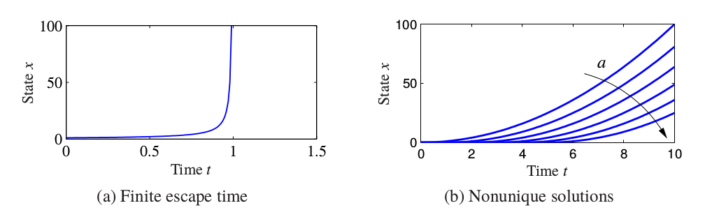
A unique solution may not always exist for all time!
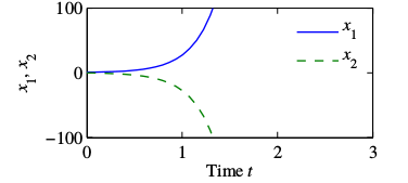
Ex 4.2 Finite escape time: \(\dot x = x^2 \) with \(x(0)=1\) yields \(x(t) = \frac{1}{1-t}\), which limits to \(\infty\) as \(t\to 1\)
Ex 4.3 Nonunique solution: \(\dot x = 2\sqrt{x} \) with \(x(0)=0\) yields
\(x(t) = \begin{cases} 0 & 0\leq t\leq a\\ (t-a)^2 & t\geq a \end{cases}, \)
for any \(a\geq 0\)
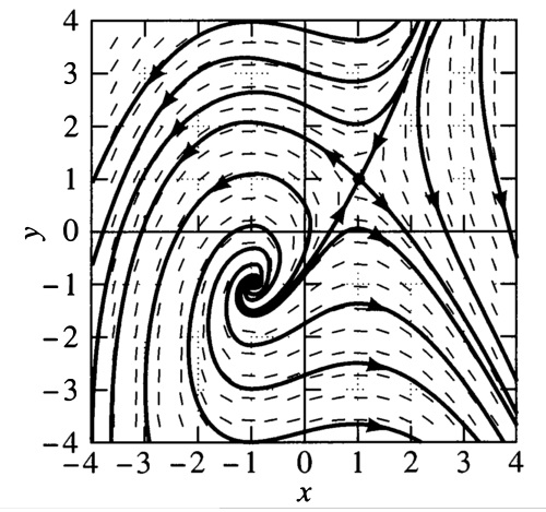
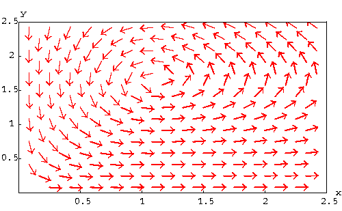
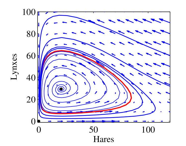
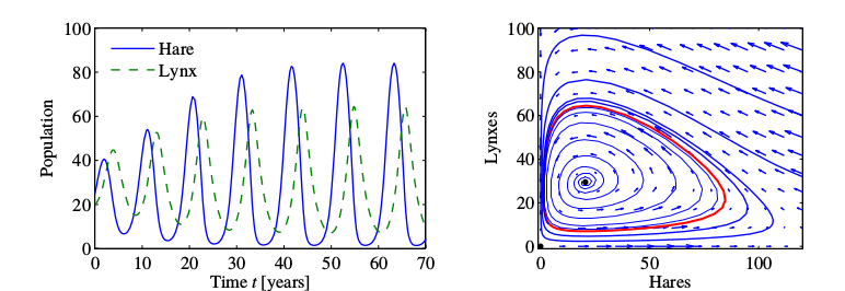
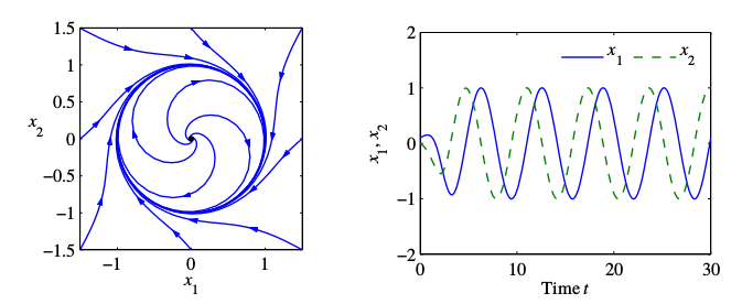
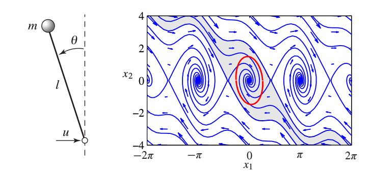
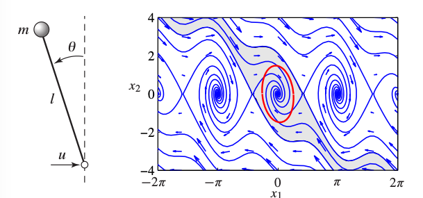
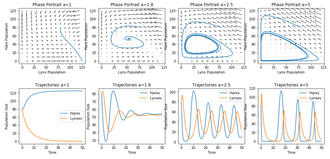
We can visualize solutions to 2D differential equations for many initial conditions
Vector fields plot the direction \(F(x)\) at each point.
Phase plots trace solutions for several initial conditions.
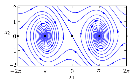
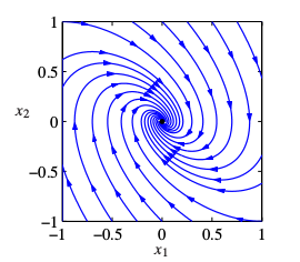
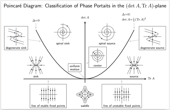
Different types of equilibrium points
Qualitatively, we observe
movement
no movement
an equilibrium point occurs when
\(\dot x = F(x) = 0\)
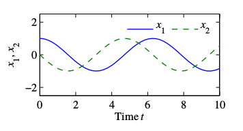
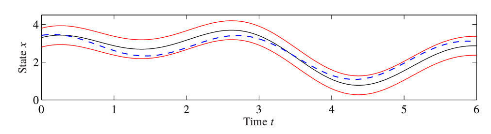
Solutions can be oscillatory, i.e. \(x(t+T)=x(t)\) for some \(T>0\)
A solution \(x(t;a)\) is stable in the sense of Lyapunov (neutrally stable) if
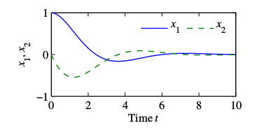
A solution is asymptotically stable if it is neutrally stable and
We can define notions of local vs. global stability
Equilibrium points that are not stable are unstable
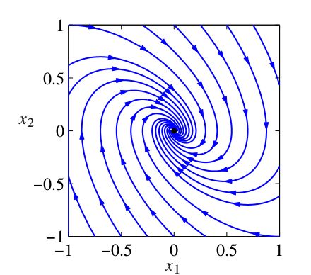
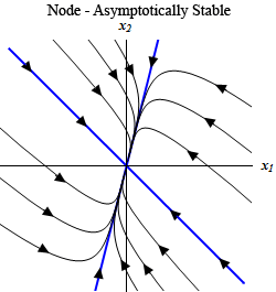
Asymptotically Stable:
Attractor/Sink
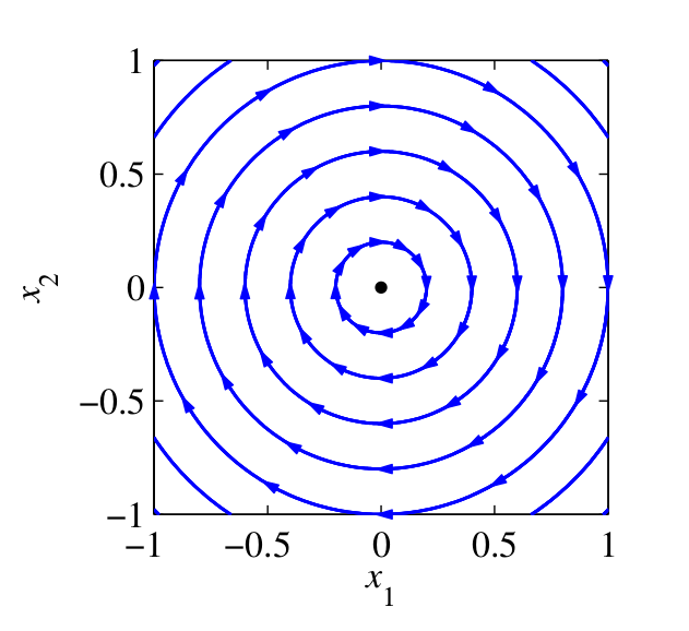
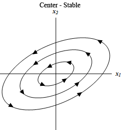
Neutrally Stable:
Center
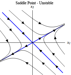
Unstable:
Source
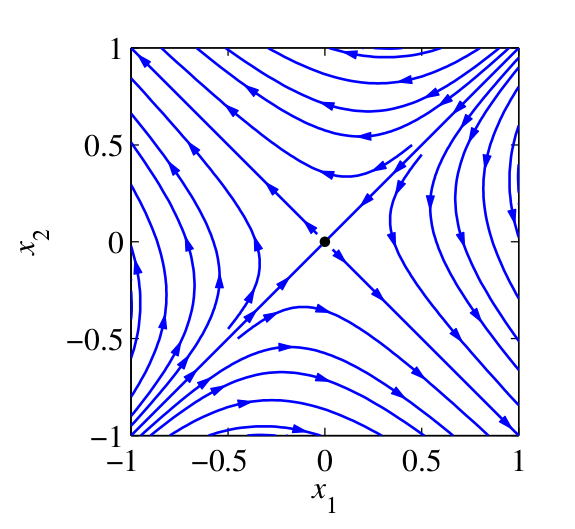
Unstable: Saddle
Why? If \(A = SDS^{-1}\), defining \(z = S^{-1} x\) gives
\( \dot z = D z \),
i.e. the system decouples \( \dot z_i = \lambda_i z_i\) and solutions are in the form
\(z_i(t) = e^{\lambda_i t}\)
Linear systems \(\dot x = A x\) have a single equilibrium at \(x=0\)
The stability is determined by the eigenvalues of \(A\):
Imaginary Eigenvalues
Real Eigenvalues
Q: What about discrete time linear systems?
A: stable when \(|\lambda(A)| < 1\), oscillatory when complex or negative
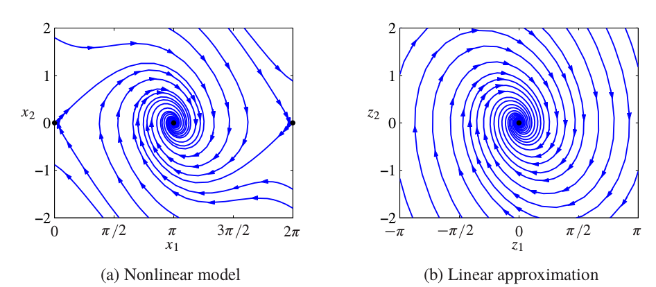
Q: Who cares about linear systems?
A: Linearization gives information about behavior of nonlinear systems near their fixed points
\(\dot x = F(x) = \cancel{F(x_{eq})} + \frac{\partial F}{\partial x}\Big |_{x_{eq}} (x - x_{eq}) \) + higher order terms
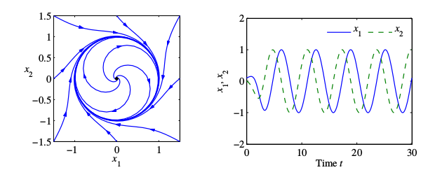
Linearization can be a useful strategy to show even complex behaviors like limit cycles.
Ex. 4.8 \( \dot x_1 = x_2 + x_1(1-x_1^2 - x_2^2),~~ \dot x_2 = -x_1 + x_2(1-x_1^2-x_2^2) \)
Polar coordinates: \(x_1 = r \cos \theta,~x_2 = r \sin \theta\) yields decoupled
\( \dot r = r(1-r^2),~~\dot \theta = -1\)
Then we can show that \(r=1\) is asymptotically stable and \(\theta(t) = \theta(0) - t\)
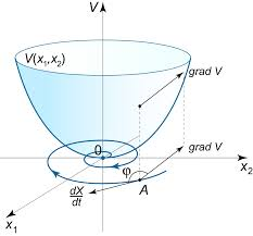
A Lyapunov function is an energy-like function that is
Lyapunov Stability Theorem:
If \(V\) is a nonnegative function such that for \(x\) in some ball,
then \(x=0\) is locally (asymptotically) stable
If \(\dot x = Ax\), then \(V(x) = x^\top P x\) is a Lyapunov function iff \(P\succ 0\) and
It is always possible to find a quadratic Lyapunov function for stable \(A\)
The Lyapunov function will be valid for all \(x\), meaning global stability
linear equation
This idea applies to more than just linear systems:
\(\dot x = Ax + \tilde F(x)\)
\(\implies \)Then we have shown local asymptotic stability for this equilibrium of the nonlinear system
This strategy will always work when
\(\|\tilde F(x) \|/\|x\| \to 0\) as \(x\to 0\)
which follows from Taylor expansion (higher order terms)
This principle allows us to show asymptotic stability even for positive semidefinite \( V\)
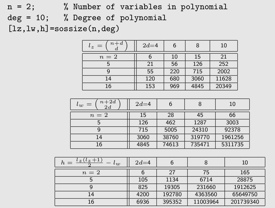
More complex forms of Lyapunov functions can be computed through sum-of-squares methods, but complexity is limited by computation
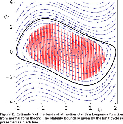
Lyapunov functions give inner approximations to regions of attraction
The region of attraction for a stable equilibrium point is the set of initial conditions that converge to it
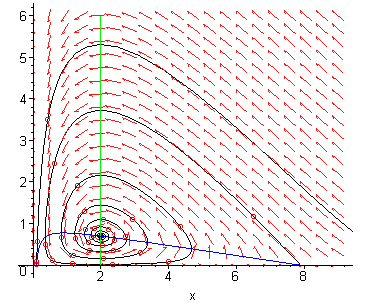
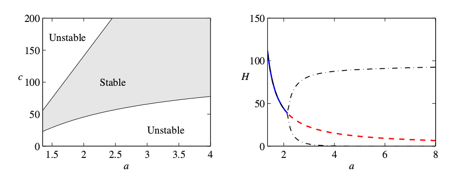
Qualitative system behavior depends on parameters of dynamic model
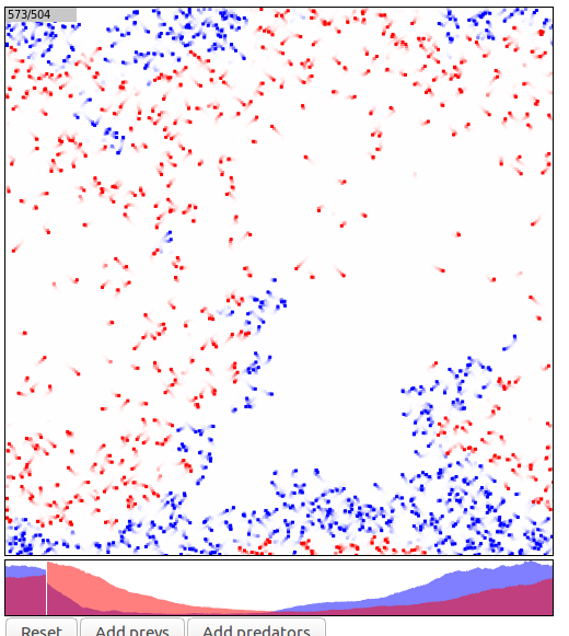
Predator-prey interactions occur stochastically and at an individual level.
A simple ODE describes qualitative behavior.
What other phenomena can be modeled in this way?
These ecological models have been used elsewhere:
Goodwin’s "class struggle model":
A growth cycle. Goodwin, 1982.
Technological adoption, stock market
Predator-Prey: An Efficient-Markets Model of Stock Market Bubbles and the Business Cycle. Gracia, 2004.
Analysis of the Lotka–Volterra competition equations as a technological substitution model. Morris and Pratt, 2003.
Interpersonal cooperation/competition
Computer simulation for exploring theories: Models of interpersonal cooperation and competition. Leik and Meeker, 1995.
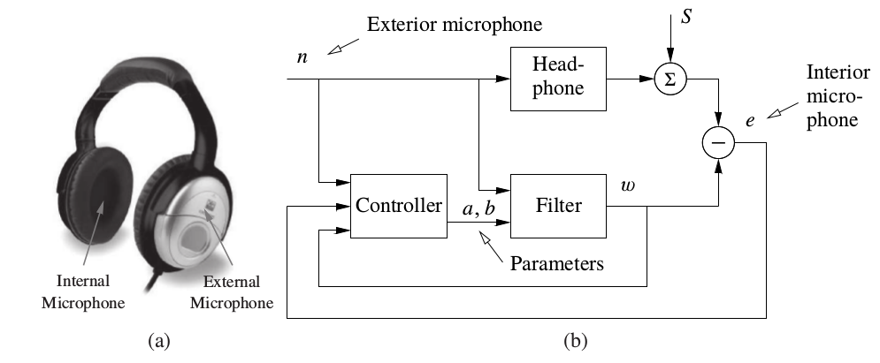
Noise cancelling headphones: adaptively update filter parameters via Lyanpunov stability analysis:
\(\dot a = -\alpha w (w-z)\) and \(\dot b = -\alpha n (w-z)\)
Today we talked about
Most of the discussion focused on closed-loop systems rather than control design!
Discussion points
By Sarah Dean


