

Sarah Dean PRO
asst prof in CS at Cornell
Interplay between these steps: online learning, exploration, adaptivity
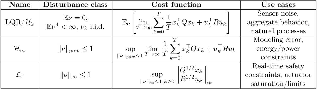
minimize \(\lim_{T\to\infty} \frac{1}{T} \sum_{t=0}^\infty \mathbb{E} [x_t^\top Q x_t + u_t^\top R u_t] \)
such that \(x_{t+1} = A_\star x_t + B_\star u_t + w_t\)
Classic optimal control problem
Static state feedback solution, \(u_t = K_\star x_t\) arises from DARE(\(A_\star,B_\star,Q,R\))
Dynamics learned by least squares:
\(\widehat A, \widehat B = \arg\min \sum_{k=0}^T \|x_{k+1} - Ax_k - Bu_k\|^2\)
\( = \arg\min \|X-Z[A~B]^\top \|_F^2\)
\(= [A_\star~B_\star]^\top + (Z^\top Z)^{-1} Z^\top W\)
\(z_k = \begin{bmatrix} x_k\\u_k\end{bmatrix}\)
Simplifying error bound relies on non-asymptotic statistics
\(\|[\widehat A-A_\star~~\widehat B-B_\star]\|_2 \leq \frac{\|Z^\top W\|_2}{\lambda_{\min}(Z^\top Z)}\)
The robust control problem:
minimize \(\max_{A,B} ~\lim_{T\to\infty} \frac{1}{T} \sum_{t=0}^\infty \mathbb{E} [x_t^\top Q x_t + u_t^\top R u_t] \)
such that \(x_{t+1} = A x_t + B u_t + w_t\)
and \(\|A-\widehat A\|_2\leq\varepsilon_A,~ \|B-\widehat B\|_2\leq\varepsilon_B\)
Any method for solving yields upper bounds on stability and realized performance, but we also want suboptimality compared with \(K_\star\)
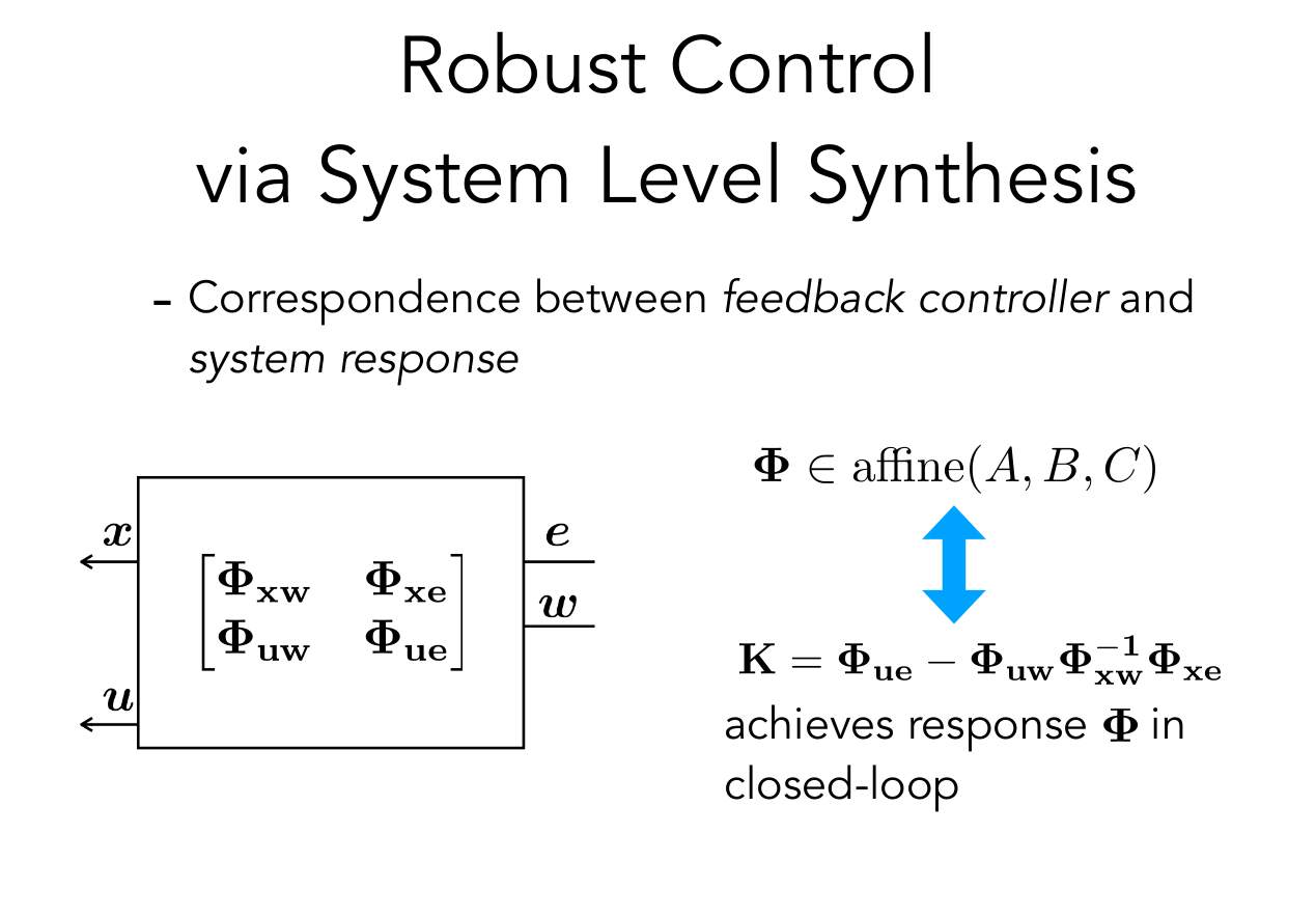
We can map planned trajectories to realized trajectories under mismatches in dynamics
\(\begin{bmatrix} \widehat{\mathbf x}\\ \widehat{\mathbf u}\end{bmatrix} = \mathbf{\widehat{\Phi} w} \)
\(\begin{bmatrix} {\mathbf x}\\ {\mathbf u}\end{bmatrix} = \mathbf{\widehat{\Phi}}(I - \mathbf{\widehat \Delta})^{-1}\mathbf w \)
\(\bf x\)
\(\bf u\)
\(\bf w\)
plant \((A,B)\)
controller \(\mathbf{K}\)
\(\bf x\)
\(\bf u\)
\(\bf w\)
robust cost
nominal achievable subspace
\( \underset{\mathbf{\Phi},\gamma}{\min}\) \(\frac{1}{1-\gamma}\)\(\text{cost}(\mathbf{\Phi})\)
\(\text{s.t.}~\begin{bmatrix}zI- \widehat A&- \widehat B\end{bmatrix} \mathbf\Phi = I\)
\(\|[{\varepsilon_A\atop ~} ~{~\atop \varepsilon_B}]\mathbf \Phi\|_{H_\infty}\leq\gamma\)
sensitivity constraints
quadratic cost
achievable subspace
minimize \(\mathbb{E}[\)cost\((x_0,u_0,x_1...)]\)
s.t. \(x_{t+1} = Ax_t + Bu_t + w_t\)
minimize cost(\(\mathbf{\Phi}\))
s.t. \(\begin{bmatrix}zI- A&- B\end{bmatrix} \mathbf\Phi = I\)
quadratic cost
achievable subspace
minimize \(\mathbb{E}[\)cost\((x_0,u_0,x_1...)]\)
s.t. \(x_{t+1} = Ax_t + Bu_t + w_t\)
minimize cost(\(\mathbf{\Phi}\))
s.t. \(\begin{bmatrix}zI- A&- B\end{bmatrix} \mathbf\Phi = I\)
Instead of reasoning about a controller \(\mathbf{K}\),
we reason about the interconnection \(\mathbf\Phi\) directly
\(\bf x\)
\(\bf u\)
\(\bf w\)
plant \((A,B)\)
controller \(\mathbf{K}\)
\(\bf x\)
\(\bf u\)
\(\bf w\)
As long as \(T\) is large enough, then w.p. \(1-\delta\),
subopt. of \(\widehat{\mathbf K}\lesssim \frac{\sigma_w C_u}{\sigma_u} \sqrt{\frac{(n+d)\log(1/\delta)}{T}} \|\)CL\((A_\star,B_\star, K_*)\|_{H_\infty} \)
Extensions
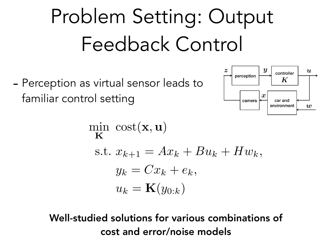
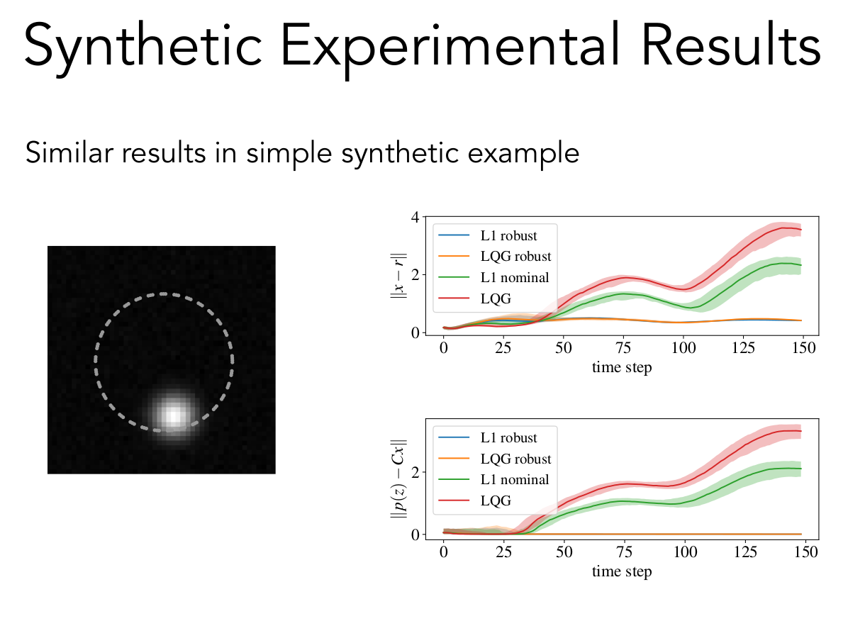
Difficulty making use of complex sensing modalities
Example: cameras on drones
Traditional Approach
End-To-End Approach
minimize \(\mathrm{cost}(\mathbf x, \mathbf u)\)
such that \(x_{k+1} = f(x_k, u_k, w_k),~~z_k = g(x_k,\nu_k),~~u_k = \gamma_k(z_{0:k})\)
Traditional State Estimation:
minimize \(\mathrm{cost}(\widehat{\mathbf x}, \mathbf u)\)
such that \(\widehat x_{k+1} = f(\widehat x_k, u_k, w_k), \\ u_k = \gamma(\widehat x_k)\)
End-to-end:
minimize \(\mathrm{cost}\)
such that \(u_k = \gamma_k(z_{0:k})\)
Our Approach: Use perception map
minimize \(\mathrm{cost}(\mathbf x, \mathbf u)\)
such that \(x_{k+1} = f(x_k, u_k, w_k),~~z_k = g(x_k,\nu_k),\)
\(u_k = \gamma_k(y_{0:k}),~~y_k=p(z_k)\approx Cx_k\)
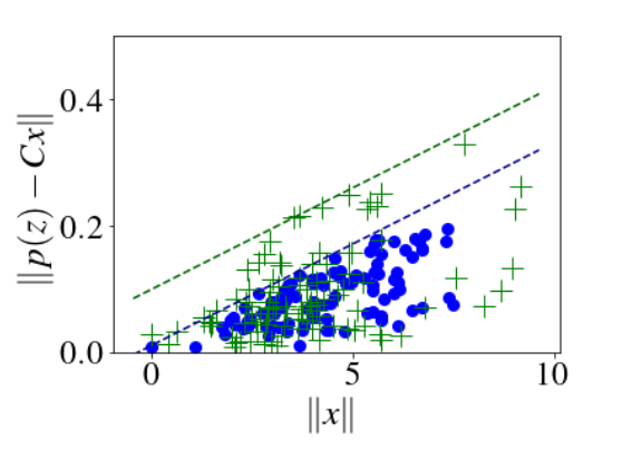
We need to fit some \(p\) and then guarantee something useful about errors \(e=Cx-p(z)\).
Robust regression:
minimize \(\varepsilon_e + \lambda R(p)\)
such that \(\|p(z_k) - x_k\|\leq \varepsilon_e\)
More generally, the errors might be better characterized as
\(p(z_k) - Cx_k = \Delta(x_k) + n_k = \Delta_{C,k} x_k + n_k\)
where \(\Delta_C\) and \(n\) are norm bounded.
Regressing error profile:
minimize \(M\varepsilon_C +\varepsilon_n\)
such that \(\|p(z_k) - x_k\|\leq \varepsilon_C\|x_k\| + \varepsilon_n\)
If we know that \(\|p(z_k) - Cx_k\|= \|e_k\|\leq \varepsilon_e\), we can apply our favorite robust control cost
The SLS problem looks like:
minimize \( \Big \| \begin{bmatrix}Q^{1/2} &\\&R^{1/2}\end{bmatrix} \mathbf{\Phi} \begin{bmatrix}\sigma_w H \\ \varepsilon_e I\end{bmatrix} \Big \| \)
such that \(\mathbf{\Phi} \in \mathrm{affine}(A,B,C)\)
Instead: \(p(z_k) - x_k=\Delta_{C,k}x_k + n_k\) for \( \|\Delta_C\| \leq \varepsilon_C\) and \(\|n\| \leq \varepsilon_n\)
Adapt the previous approach to handle uncertainty in the sensing matrix.
The robust SLS problem looks like:
minimize \( \Big \| \begin{bmatrix}Q^{1/2} &\\&R^{1/2}\end{bmatrix} \begin{bmatrix}\mathbf{\Phi_{xw}} & \mathbf{\Phi_{xn}} \\ \mathbf{\Phi_{uw}} & \mathbf{\Phi_{un}} \end{bmatrix} \begin{bmatrix}\sigma_w H \\ \varepsilon_n I\end{bmatrix} \Big \|\)
\(+ \frac{\varepsilon_C(\gamma\varepsilon_w + \tau\varepsilon_n)}{1-\tau\varepsilon_C}\Big \| \begin{bmatrix}Q^{1/2} \\R^{1/2}\end{bmatrix} \begin{bmatrix} \mathbf{\Phi_{xn}} \\ \mathbf{\Phi_{un}} \end{bmatrix} \Big \| \)
such that \(\mathbf{\Phi} \in \mathrm{affine}(A,B,C)\), \(\|\mathbf{\Phi_{xw}}H\|\leq \gamma\), \(\|\mathbf{\Phi_{xn}}\|\leq \tau\)
We can synthesize a controller \(\mathbf \Phi\) with performance
cost\((\mathbf \Phi)\leq \Big \| \begin{bmatrix}Q^{1/2} &\\&R^{1/2}\end{bmatrix} \mathbf{\Phi} \begin{bmatrix}\sigma_w H \\ (\widehat\varepsilon_e + \varepsilon_\mathrm{gen}) I\end{bmatrix} \Big \| \)
where \(\varepsilon_\mathrm{gen} \) depends on smoothness and robustness of the perception map, bounded closed-loop response to errors \(\mathbf\Phi_{xe}\), and the planned trajectory's distance to training points
If we learn some perception map \(p\) and error bound \(\widehat \varepsilon_e\) on training data, what can we say about the performance of \(p\) during operation?
Non-parametric guarantees from learning theory on risk \(\mathcal R\)
\( \mathcal R(p) = \mathcal R_N(p) +\mathcal R(p)- \mathcal R_N(p) \leq \mathcal R_N(p) +\varepsilon_\mathrm{gen} \)
e.g. for classic ERM, \( \mathbb{E}_{\mathcal D}[\ell(p;x,z)] \leq \mathbb{E}_{\mathcal D_N}[\ell(p;x,z)] + \mathcal{O}(\sqrt{\frac{1}{N}})\)
This usual statistical generalization argument relies on \(\mathcal D_N\) being drawn from \(\mathcal D\).
Our setting looks more like
\( \mathbb{E}_{\mathcal D}[\ell(p;x,z)] = \mathbb{E}_{\mathcal D_N'}[\ell(p;x,z)] \)
\(+(\mathbb{E}_{\mathcal D_N}[\ell(p;x,z)]- \mathbb{E}_{\mathcal D_N'}[\ell(p;x,z)] )\)
\(+ (\mathbb{E}_{\mathcal D}[\ell(p;x,z)] - \mathbb{E}_{\mathcal D_N}[\ell(p;x,z)] ) \)
\(\leq \mathbb{E}_{\mathcal D_N'}[\ell(p;x,z)] +\varepsilon_\mathrm{shift}\rho(\mathcal{D,D'})+ \varepsilon_N\)
But our training and closed-loop distributions will be different, especially since \(\mathcal D\) depends on the errors \(\mathbf e\) themselves,
\(\mathbf x = \mathbf{\Phi_w w + \Phi_e e}\)
High level generalization argument
But our training and closed-loop distributions will be different, especially since \(\mathcal D\) depends on the errors \(\mathbf e\) themselves,
\(\mathbf x = \mathbf{\Phi_w w + \Phi_e e}\)
From this, we can bound \(\mathcal R(p) \) and \(\rho(\mathcal{D,D'}) \) as long as \(\varepsilon_\mathrm{shift}\varepsilon_\mathrm{rob}\leq 1\)
\(\implies\) guarantees on performance and stability.
We take a robust and adversarial view,
training distribution \(\mathcal D'\) specified by points \(\{(x_d,z_d)\}\), "testing" distribution \(\mathcal D\) specified by trajectory \(\mathbf x, \mathbf z\)
Then \(\mathcal{R}(p) = \|C\mathbf x - p(\mathbf z)\| \), \(\mathcal{R}_N(p) = \max_k \|Cx_k - p(z_k)\| \), and \(\rho(\mathcal{D,D'}) = \min_{\mathbf x_d}\|\mathbf{x-x_d}\|\)
In lieu of distributional assumptions, we assume smoothness.
This is possible as long as \(L_e\|\mathbf{ \Phi_{xe}}\|\leq 1\)
Design controller to remain within set:
For example, with reference tracking:
\(\|\)\(\mathbf{x_\mathrm{ref}}\)\(-\mathbf{x_d}\|+\|\mathbf{ \Phi_{xw}}H\|\varepsilon_\mathrm{ref}\)
Controller design balances responsiveness to references \(\|\mathbf{ \Phi_{xw}}H\|\) with sensor response \(\|\mathbf{ \Phi_{xe}}\|\)
We can synthesize a controller \(\mathbf \Phi\) with performance
cost\((\mathbf \Phi)\leq \Big \| \begin{bmatrix}Q^{1/2} &\\&R^{1/2}\end{bmatrix} \mathbf{\Phi} \begin{bmatrix}\sigma_w H \\ (\widehat\varepsilon_e + \varepsilon_\mathrm{gen}) I\end{bmatrix} \Big \| \)
where \(\varepsilon_\mathrm{gen} \) depends on smoothness \(L_e\) and robustness \(\varepsilon_p\) of the perception map, bounded closed-loop response to errors \(\mathbf\Phi_{xe}\), and the planned trajectory's distance to training points \(\rho_0\).
\(\varepsilon_\mathrm{gen} = \frac{2\varepsilon_p+L_e\rho_0}{1-L_e\|\mathbf{\Phi_{xe}}\|}\)
By Sarah Dean


