


Sarah Dean PRO
asst prof in CS at Cornell
L4DC, 8 June 2021
Machine learning is a promising avenue for incorporating rich sensing modalities
Can we make strong guarantees in these settings?
backup slide about EKF/modelling vs. end-to-end
\(\displaystyle \min_{\pi\in\Pi} ~~\mathrm{cost}(x_0,u_0,x_1,\dots)\)
\(~~~\mathrm{s.t.}~~ u_t = \pi_t(z_{0:t})\)
\(~~~~~~~~~~x_{t+1} = \mathrm{dynamics}_t(x_t,u_t)\)
\(~~~~~~~~~~z_t = \mathrm{observation}_t(Cx_t)~\)
observation
?
?
\(\mathrm{dynamics~\&}\)\(\mathrm{observation}\)
\(\pi\)
\(z_t\)
\(u_t\)
\(x_t\)
output
\(y_t=Cx_t\)
Observation-feedback optimal control problem
\(\displaystyle \min_{\pi\in\Pi} ~~\mathrm{cost}(\widehat x_0,u_0,\widehat x_1,\dots)\)
\(~~~\mathrm{s.t.}~~ u_t = \pi_t(\widehat x_{0:t})\)
\(~~~~~~~~~~\widehat x_{t+1} = \mathrm{dynamics}_t(\widehat x_t,u_t)\)
\(~~~~~~~~~~\widehat x_t =\mathrm{EKF}(z_{0:t})~\)
\(\mathrm{dynamics,}\)\(\mathrm{obs, EKF}\)
\(\pi\)
\(\widehat x_t\)
\(u_t\)
\(x_t\)
Classic approach: physical models and filtering
\(\displaystyle \min_{\pi\in\Pi} ~~\mathrm{cost}(x_0,u_0,x_1,\dots)\)
\(~~~\mathrm{s.t.}~~ u_t = \widehat \pi_t(z_{0:t})\)
?
\(\mathrm{dynamics~\&}\)\(\mathrm{observation}\)
\(\widehat \pi\)
\(z_t\)
\(u_t\)
\(x_t\)
End-to-end approach: learn everything from data
\(\displaystyle \min_{\pi\in\Pi} ~~\mathrm{cost}(x_0,u_0,x_1,\dots)\)
\(~~~\mathrm{s.t.}~~ u_t = \pi_t(y_{0:t})\)
\(~~~~~~~~~~x_{t+1} = \mathrm{dynamics}_t(x_t,u_t)\)
\(~~~~~~~~~~y_t = \mathrm{perception}(\mathrm{observation}_t(Cx_t))~\)
\(\mathrm{dynamics~\&}\)\(\mathrm{obs,~percept.}\)
\(\pi\)
\(y_t\)
\(u_t\)
\(x_t\)
Our focus: learned perception map
\(\text{s.t.}~~x_{t+1} = {A }x_t+ {B} u_t\)
Robust reference tracking with linear dynamics and nonlinear partial observation
\(z_{t} =g(Cx_t)\)
\(\displaystyle\mathrm{cost} = \sup_{\substack{t\geq 0\\\mathbf x^\mathrm{ref} \in \mathcal R\\ \|x_0\|\leq \sigma_0}}\left\|\begin{bmatrix} Q (x_t - x_t^\mathrm{ref})\\ Ru_t \end{bmatrix}\right\|_\infty\)
Assumption 1:
\(A,B,C\) and \(Q,R\) are known and well posed
Assumption 2:
\(\mathcal R\) encodes a bounded radius of operation
Assumption 3:
Invertible \(h(g(y)) = y\) and \(g,h\) continuous
\(\displaystyle \min_{\pi}\)
\(\displaystyle \min_{\mathbf K}\)
\(u_{t} =\pi(z_{0:t}, x^\mathrm{ref}_{0:t})\)
Assumption 4:
Noisy training signal \(y^\mathrm{train}_{t} =Cx_t+\eta_t\)
\(y_t = h(z_t) = Cx_t\)
\(u_t = \mathbf K(y_{0:t}, x^\mathrm{ref}_{0:t})\)
Certainty equivalent controller \(\widehat \pi(z_{0:t}, x^\mathrm{ref}_{0:t}) = \mathbf K_\star (\widehat h(z_{0:t}), x^\mathrm{ref}_{0:t}) \)
where \(\widehat h\) is learned from data
Transform to linear output feedback problem with \(h\)
\(\pi_\star(z_{0:t}, x^\mathrm{ref}_{0:t}) = \mathbf K_\star (h(z_{0:t}), x^\mathrm{ref}_{0:t}) \)
Assumption 3 applies when:
\(\mathrm{dynamics~\&}\)\(\mathrm{observation}\)
\(\mathbf K\)
\(z_t\)
\(u_t\)
\(x_t\)
\(y_t\)
\(\mathrm{linear}\)
\(\mathrm{dynamics}\)
\(\mathbf K\)
\(y_t\)
\(u_t\)
\(x_t\)
\(h\)
\(\mathrm{cost}(\widehat\pi) - \mathrm{cost}(\pi_\star) \lesssim\) \( L \) \(r_\star\) \(s_\star\) \( \left(\frac{\sigma}{T}\right)\)\({}^{\frac{1}{p+4}}\)
depending on the continuity of \(g\) and \(h\), the radius of operation, the sensitivity of the optimal controller, the sensor noise, amount of data, and the dimension of the output
Ingredients
The certainty-equivalent controller has bounded suboptimality w.h.p.
1. Uniform convergence of \(\widehat h\)
2. Closed-loop performance
Classic controls: Weiner system identification
Recent work:
Block MDP (Misra et al. 2020) and Rich LQR (Mhamedi et al. 2020) settings
Example: 1D unstable linear system with arbitrary linear controller
\(x_{t+1} = a x_t + u_t\qquad u_t = \mathbf{K}(x^\mathrm{ref}_{0:t},\widehat h(z_{0:t}))\)
near perfect perception map: \(\widehat h(g(x)) = \begin{cases} 0 & x = \bar x,~ |x|>r\\ x &\text{otherwise} \end{cases}\)
There exists a reference signal contained in \([-r,r]\) that causes the system to pass through \(\bar x\) and subsequently go unstable
\(\bar x\)
\(r\)
\(-r\)
\(t\)
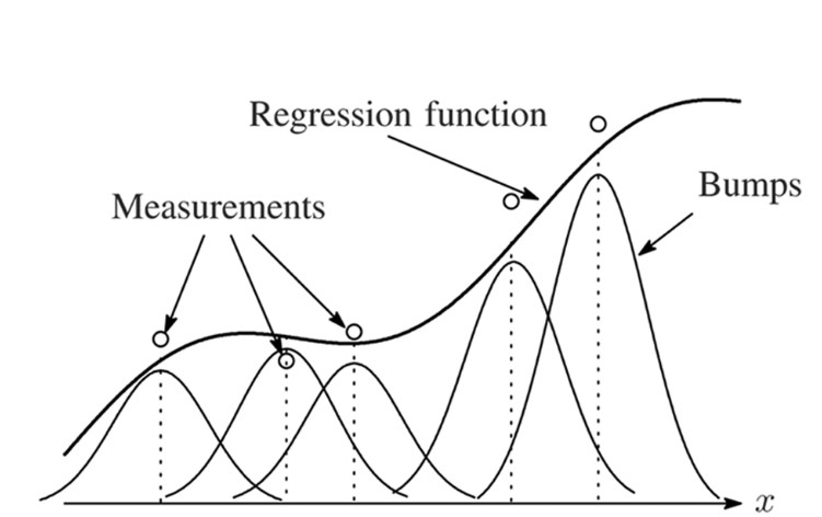
Nadarya Watson Regression: from training data \(\{(z_t, y_t^\mathrm{train})\}_{t=0}^T\)
predictions are weighted averages,
\(\displaystyle \widehat h(z) = \sum_{t=0}^T \frac{k_\gamma(z_t, z)}{\sum_{\ell=0}^T k_\gamma(z_\ell, z)} y_t^\mathrm{train} \)
Theorem (uniform convergence): Suppose training data uniformly sampled from \( \{y\mid \|y\|_\infty\leq r\}\) and bandwidth \(\gamma \propto T^{\frac{1}{p+4}}\). Whenever the system state contained in \(\{x\mid\|Cx\|_\infty \leq r\}\), then w.h.p.
\(\|h(z) - \widehat h(z)\|_\infty \lesssim rL_g L_h \left(\frac{p^2\sigma_\eta^4}{T}\right)^{\frac{1}{p+4}}\)
bandwidth
Nadarya Watson Regression: from training data \(\{(z_t, y_t^\mathrm{train})\}_{t=0}^T\)
\(\displaystyle \widehat h(z) = \sum_{t=0}^T \frac{k_\gamma(z_t, z)}{s_T(z)} y_t^\mathrm{train} \)
\(=\sum_{t=0}^T k_\gamma(z_t, z)\)
The kernel function has the form \(\kappa\left(\frac{\rho(z_t, z)}{\gamma}\right)\) for
Drive system to uniform samples \(y_\ell^\mathrm{ref}\) using training output \(y_t^\mathrm{train}\)
\(\mathbf K\)
\(y^\mathrm{ref}_\ell \sim \mathrm{Unif}\{|y|\leq r\}\)
\(\mathrm{dynamics~\&}\)\(\mathrm{observation}\)
\(z_t\)
\(u_t\)
\(x_t\)
\(y_t^\mathrm{train}\)
How to achieve uniform sampling?
How does imperfect perception affect system evolution?
Define errors \(e_t = \widehat h(z_t) - h(z_t) = \widehat h(z_t) - Cx_t\)
\(\displaystyle u_t = \sum_{k=0}^t K_k^y \widehat h(z_{t-k}) + K_k^\mathrm{ref} x^\mathrm{ref}_{t-k}\)
\(\displaystyle x_{t+1}=Ax_t+Bu_t\)
\(\displaystyle u_t = \sum_{k=0}^t K_k^y Cx_{t-k} + K_k^y Ce_{t-k} + K_k^\mathrm{ref} x^\mathrm{ref}_{t-k}\)
\(x_t = \sum_{k=0}^t \Phi_{xe}(k) e_{t-k} + \Phi_{xr}(k) x^\mathrm{ref}_{t-k}\)
Linearly.
\(u_t = \sum_{k=0}^t \Phi_{ue}(k) e_{t-k} + \Phi_{ur}(k) x^\mathrm{ref}_{t-k}\)
Proposition: Suppose that perception errors are uniformly bounded by \(\varepsilon_h\) and let \(\mathbf \Phi\) be system response associated with \(\mathbf K_\star\). Then,
\(\mathrm{cost}(\widehat\pi) \leq \mathrm{cost}(\pi_\star) + \varepsilon_h ~\left\|\begin{bmatrix} Q\mathbf \Phi_{xe}\\ R\mathbf \Phi_{ue} \end{bmatrix}\right\|_{\mathcal L_1} \)
\(\mathrm{cost}(\widehat\pi) - \mathrm{cost}(\pi_\star) \lesssim\) \(rL_g L_h \left(\frac{p^2\sigma_\eta^4}{T}\right)^{\frac{1}{p+4}}\) \(\left\|\begin{bmatrix} Q\mathbf \Phi_{xn}\\ R\mathbf \Phi_{un} \end{bmatrix}\right\|_{\mathcal L_1} \)
The certainty-equivalent controller has bounded suboptimality w.h.p.
Ingredients
1. Uniform convergence of \(\widehat h\)
bounded errors
2. Closed-loop performance
propagation of errors
Simplified UAV model: 2D double integrator
\(x_{t+1} = \begin{bmatrix}1 & 0.1 & & \\ 0 & 1 & & \\ & & 1 & 0.1 \\ & & 0 & 1\end{bmatrix} x_t +\begin{bmatrix}0 & \\ 1 & \\ & 0 \\ & 1 \end{bmatrix} u_t \)
\(y_t = \begin{bmatrix} 1 & 0 & & \\ & & 1 & 0\end{bmatrix} x_t\)
\(z_t\) from CARLA simulator
Data collected with linear control and periodic reference signal:
Nadarya Watson (NW) with kernel \(k_\gamma(z, z_t) = \mathbf{1}\{\|z-z_t\|_2 \leq \gamma\}\)
Kernel Ridge Regression (KRR) with radial basis functions
Visual Odometry (VO) matches \(z\) to some \(z_t\) in database of labelled training images, uses homography between images to estimate pose
Simultaneous Localization and Mapping (SLAM) like VO with memory: adds new observations to database online, and initializes estimates based on previous timestep
classic nonparametric methods look similar
memoryless classic computer vision is similar, if noisier/wider
very different!
building obstructs view
Certainty-Equivalent Perception-Based Control
Sarah Dean and Benjamin Recht
Read more at arxiv.org/abs/2008.12332
Code at github.com/modestyachts/certainty_equiv_perception_control
By Sarah Dean


