Thesis Defence on Weather Forecasting with Data-Driven Models and Sequential Data Assimilation
Presented by: Bsc. Sebastian David Ariza Coll
Advisor: Elias David Niño Ruiz, PhD.
Content
- Introduction
- Objectives
- Background
- Numerical Experiments
- Conclusions and future works
Introduction
- Weather forecasting (WF) is a crucial domain attracting significant attention across diverse research communities due to its global ramifications.
- The exponential growth in weather observation data and advancements in information technology compel researchers to unearth concealed patterns within extensive datasets to enhance prediction accuracy.
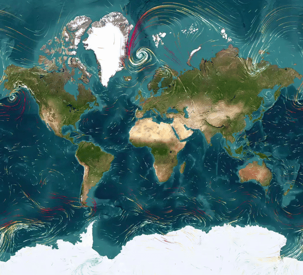
Hurricane Katrina wind speed, forecasts made by NOAA
- This field holds immense potential for various sectors such as aviation, agriculture, tourism, and energy production.
- However, it confronts challenges in processing vast datasets and constructing robust prediction models to discern underlying patterns.
- Over the past decade, considerable strides have been made, notably through the application of statistical modeling techniques, including machine learning
Statistical modeling techniques
Objectives
General
Specifics
To implement efficient formulation of data-driven models to make weather forecast and improve this one via sequential data assimilation.
- To implement an efficient parameter optimizer for data-driven methods for weather forecast.
- To implement an efficient data assimilation method based on EnKF with Decorrelation matrix.
- To validate the formulations via metrics from specialized literature.
Background
Data - Driven Models
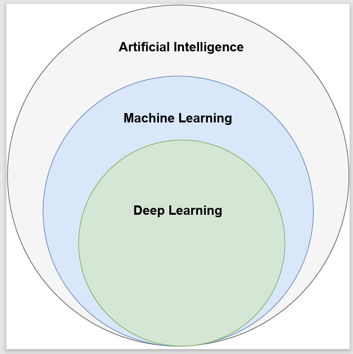
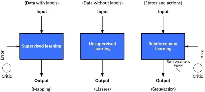
Main types of Machine Learning
Source: (Geron, 2019; Goodfellow et al.2016), https://developer.ibm.com/articles/cc-models-machine-learning/
Context of this Master's thesis
Prediction models have been developed using Autoencoders based on Convolutional Neural Networks (CNN) architectures. This type of Machine Learning is based on unsupervised training.
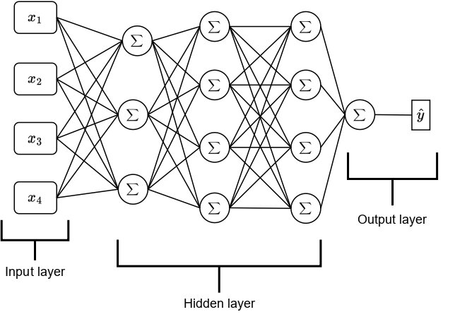
ANN Architecture
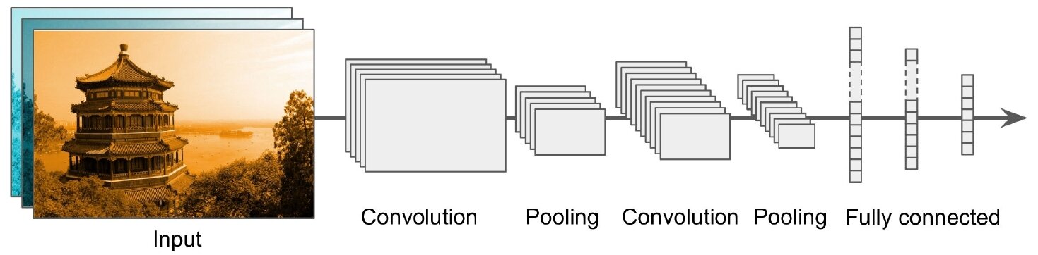
Typical CNN Architecture
The term CNNs suggests that the network employs a mathematical operation called Convolution. Convolution is a specialized form of a linear operation. Convolutional networks are essentially neural networks that utilize convolution instead of general matrix multiplication in at least one of their layers (Geron, 2019; Goodfellow et al., 2016).
Source: (Geron, 2019)
The Convolution Operation
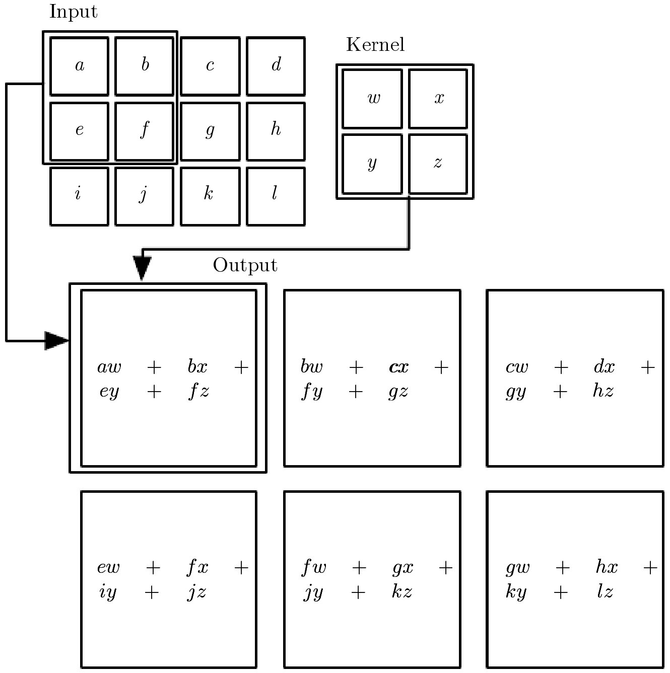
Source: (Geron, 2019)
S(i,j) = (I * K)(i,j) = \sum_{m}\sum_{n} I(m,n) K(i-m,j-n)
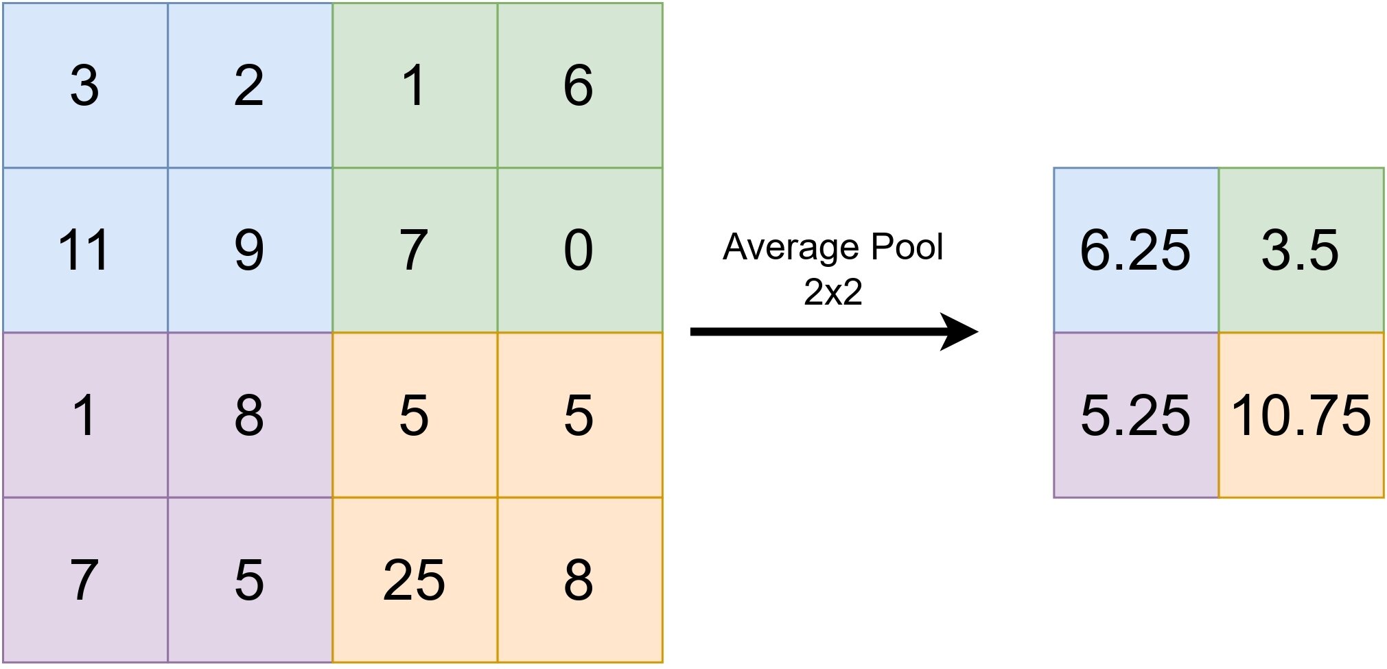
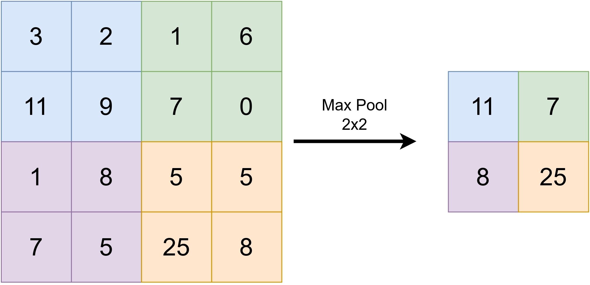
Pooling
Two fundamental pooling operations in neural networks are max-pooling and average-pooling. The choice between them depends on the specific problem under consideration. In the context of vision-related problems, max-pooling is often the preferred option. These operations could be seen as follows:
Activation Functions
Non-linear problems
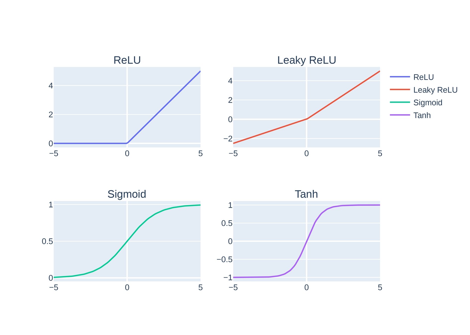
Graphs of main activation’s functions
Autoencoder
Autoencoders are neural networks aiming to learn concise data representations. They comprise an encoder mapping input to a hidden representation, and a decoder reconstructing the output. Training aims to minimize reconstruction error, often with regularization. They excel in dimensionality reduction, feature learning, and now in generative modeling and unsupervised tasks (Geron, 2019; Goodfellow et al., 2016; Ng et al., 2011).
Convolucional autoencoder

ANN Autoencoder
Data Assimilation
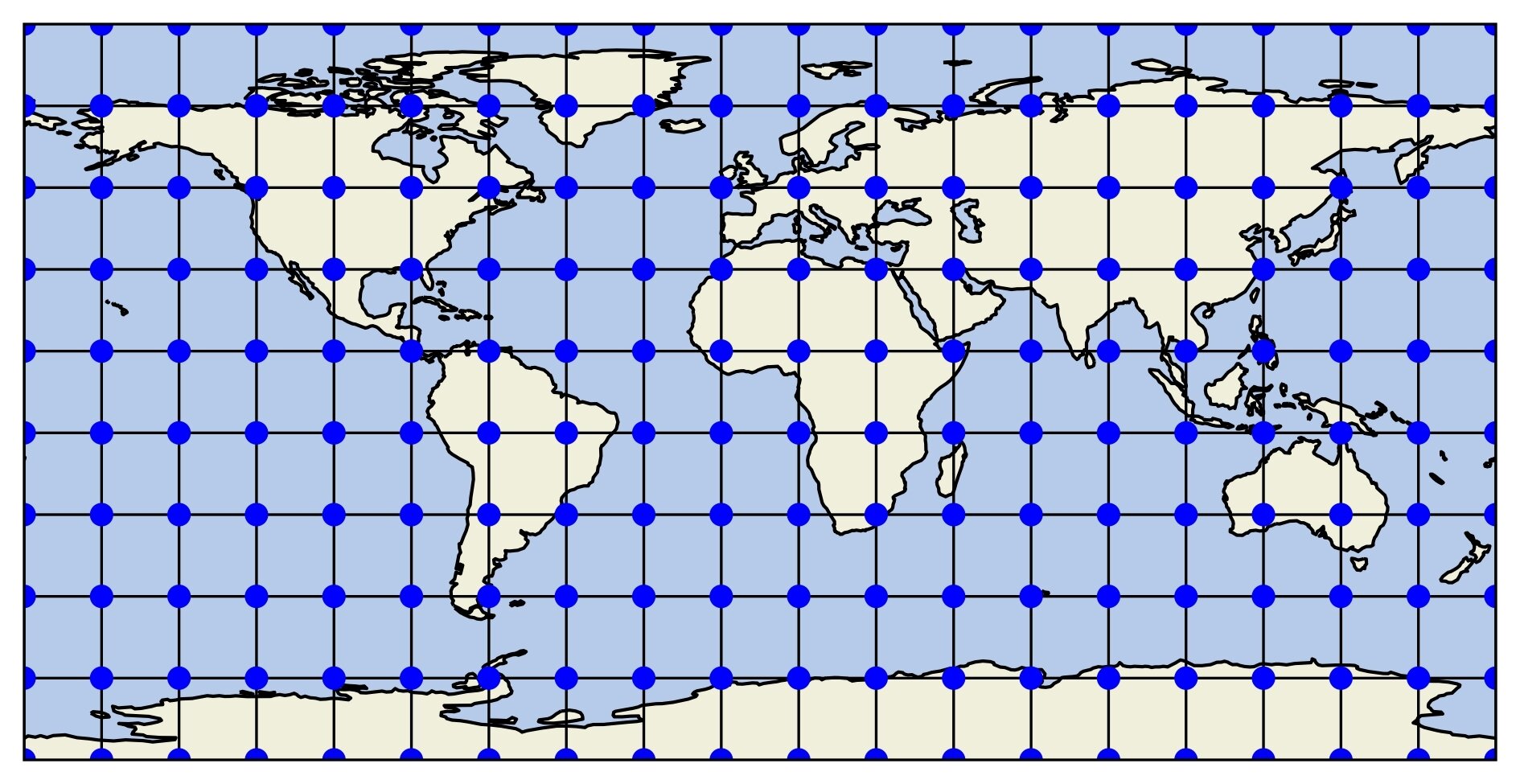
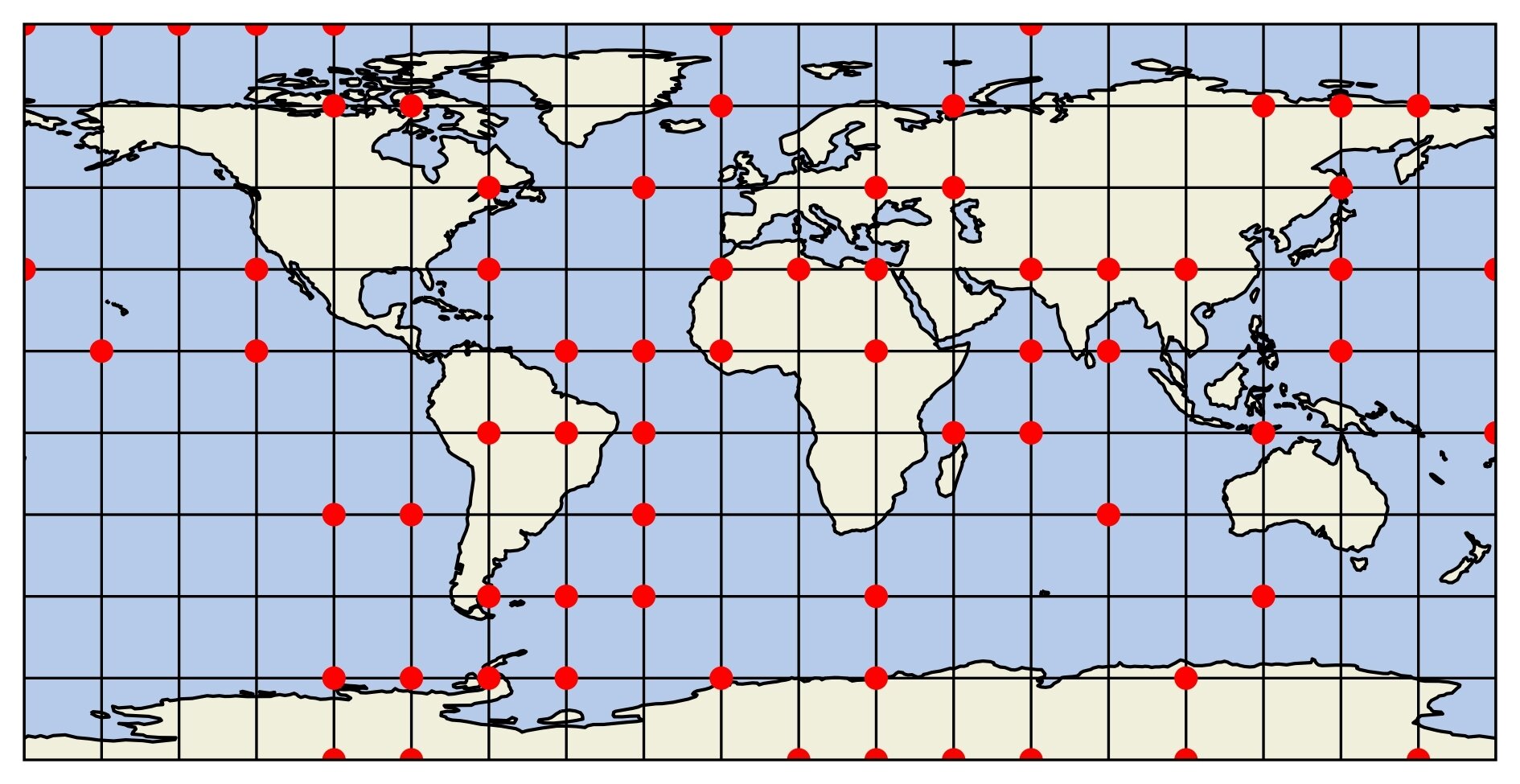
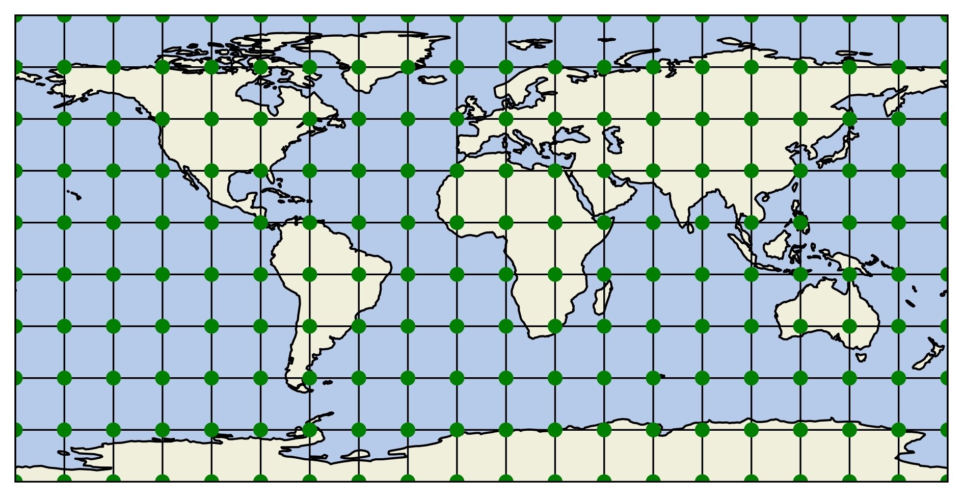
Model component
Observation space
Analysis
Data assimilation (DA) is a methodological approach aiming to enhance model predictions by integrating observational data. It addresses the need for accurate forecasts, crucially dependent on robust models. Without periodic calibration against real-world observations, models can degrade, diminishing their utility. Thus, optimizing model states to match observations is vital before analysis or prediction, a common scenario in inverse problems. DA essentially approximates a physical system's true state by merging distributed observations with a dynamic model (Asch et al., 2016; Lahoz et al., 2010; McLaughlin, 2014; Vetra-Carvalho et al., 2018)
Bayesian Framework
In Statistical Data Assimilation, the observations are assimilated into the model forecast (background) by inference (Hannart et al., 2016; Nearing et al., 2018)
\mathcal{P}(\mathbf{x} \vert \mathbf{y}) = \frac{\mathcal{P}(\mathbf{y} \vert \mathbf{x}) \cdot \mathcal{P}(\mathbf{x})}{\mathcal{P}(\mathbf{y})}
\mathcal{P}(\mathbf{y} \vert \mathbf{x}) = \mathcal{L}(\mathbf{x} \vert \mathbf{y})
\mathcal{P}(\mathbf{x})
\mathcal{P}(\mathbf{y}) = \int_{\mathbf{x}}\mathcal{P}(\mathbf{y} \vert \mathbf{x})\mathcal{P}(\mathbf{x})
\mathcal{P}(\mathbf{x} \vert \mathbf{y})
quantifies the distribution in observations error. is the maximum Likelihood.
Where:
\mathcal{L}
is the previous knowledge about system state
is the normalization constant
is the update estimation of the true state
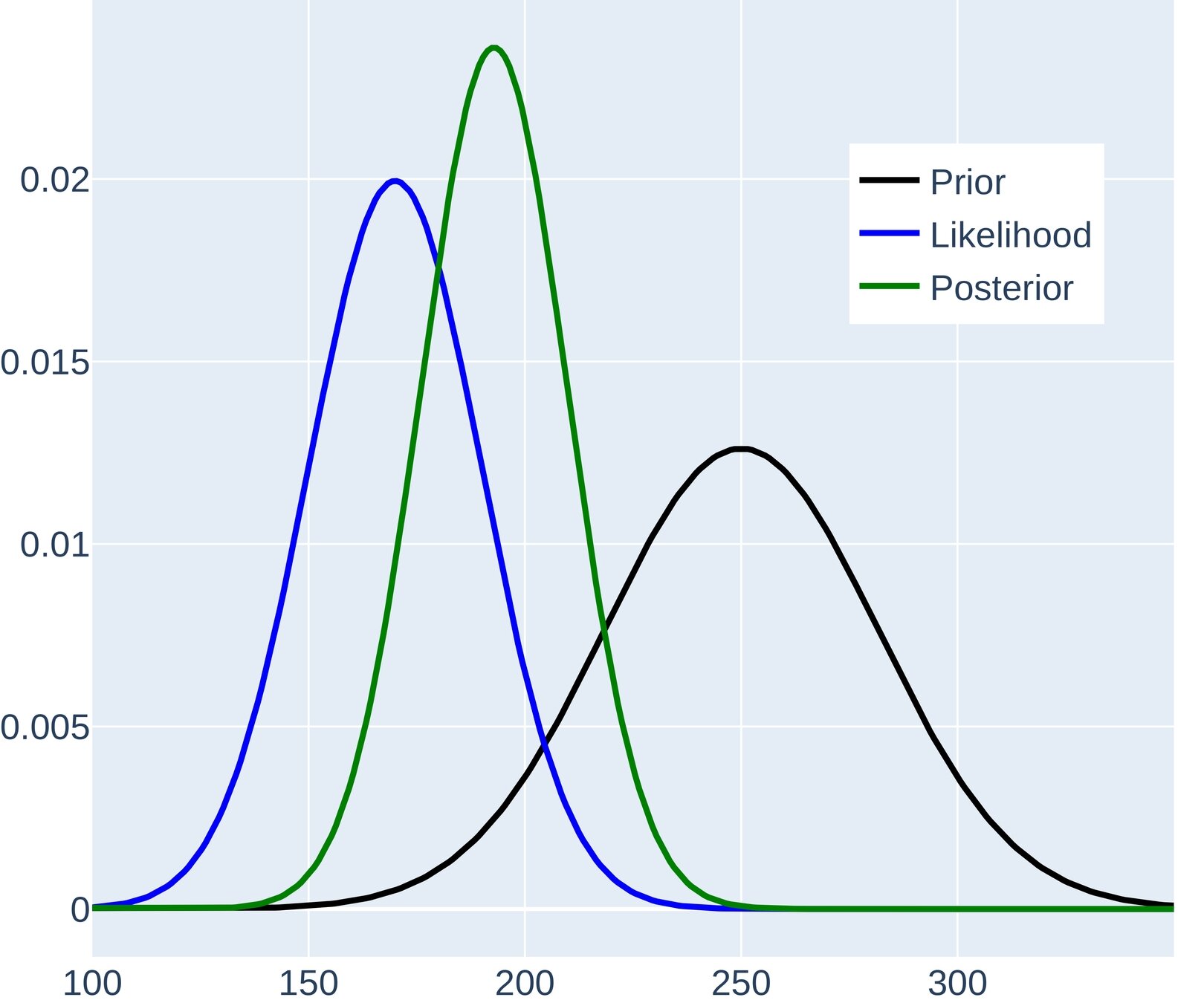
Bayesian inference - One dimension case
Statistical Data Assimilation
Based on Bayes theorem, it is completed corrected to say that
\mathcal{P}(\mathbf{x} \vert \mathbf{y}) \propto \mathcal{P}(\mathbf{y} \vert \mathbf{x}) \cdot \mathcal{P}(\mathbf{x})
Which means that model state updates are made as soon as observations are available and then the estimate is propagated. Recall the Gaussian assumption given, the inverse problem resolved to compute the analysis is the following optimization problem:
\mathbf{x}_k^a
\mathbf{x}^{*} \equiv \mathbf{x}^{a} = \operatorname*{arg\,max}_\mathbf{x} \mathcal{P}(\mathbf{x} \vert \mathbf{y})
Statistical Data Assimilation
\mathbf{x} - \mathbf{x}^{b} \sim \mathcal{N}(0,\mathbf{B}), \mathbf{B} \in \mathbb{R}^{n \times n}
is the background covariance matrix, and in general be time independent.
is independent.
is the observations covariance matrix, and in general be time independent.
\mathbf{B}^{\mathsf{T}} = \mathbf{B}.
is independent.
\delta \sim \mathcal{N}(0,\mathbf{B})
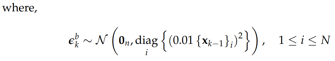
\mathbf{y} - \mathbf{H} \cdot \mathbf{x} \sim \mathcal{N}(0,\mathbf{R}), \mathbf{R} \in \mathbb{R}^{m \times m}
\epsilon \sim \mathcal{N}(0,\mathbf{R})
\mathbf{R}^{\mathsf{T}} = \mathbf{R}.
It is possible to say that:
\mathcal{P}(\mathbf{x}) = \frac{\exp{\left(-\frac{1}{2}\left\lVert\mathbf{x}-\mathbf{x}^b\right\rVert^{2}_{\mathbf{B}^{-1}}\right)}}{\sqrt{(2\pi)^{n}|\mathbf{B}|}} \propto \exp{\left(-\frac{1}{2}\left\lVert\mathbf{x}-\mathbf{x}^b\right\rVert^{2}_{\mathbf{B}^{-1}}\right)}
\mathcal{P}(\mathbf{y} \vert \mathbf{x}) = \frac{\exp{\left(-\frac{1}{2}\left\lVert\mathbf{y}-\mathbf{H} \cdot \mathbf{x}\right\rVert^{2}_{\mathbf{R}^{-1}}\right)}}{\sqrt{(2\pi)^{m}|\mathbf{R}|}} \propto \exp{\left(-\frac{1}{2}\left\lVert\mathbf{y}-\mathbf{H} \cdot \mathbf{x}\right\rVert^{2}_{\mathbf{R}^{-1}}\right)}
\mathcal{P}(\mathbf{x} \vert \mathbf{y}) \propto \exp{\left(-\frac{1}{2}\left\lVert\mathbf{x}-\mathbf{x}^b\right\rVert^{2}_{\mathbf{B}^{-1}}\right)} \cdot \exp{\left(-\frac{1}{2}\left\lVert\mathbf{y}-\mathbf{H} \cdot \mathbf{x}\right\rVert^{2}_{\mathbf{R}^{-1}}\right)}
\rightarrow \mathcal{P}(\mathbf{x} \vert \mathbf{y}) \propto \exp{\left[-\underbrace{\frac{1}{2}\left(\left\lVert\mathbf{x}-\mathbf{x}^b\right\rVert^{2}_{\mathbf{B}^{-1}} + \left\lVert\mathbf{y}-\mathbf{H} \cdot \mathbf{x}\right\rVert^{2}_{\mathbf{R}^{-1}}\right)}_{\mathcal{J}(\mathbf{x})}\right]}=\exp[{-\mathcal{J}(\mathbf{x})}]
Note that
-\ln{[\mathcal{P}(\mathbf{x} \vert \mathbf{y})]} \propto -\ln{\{\exp[{-\mathcal{J}(\mathbf{x})}]\}}
What means that the optimization problem can be written as
\mathbf{x}^{*} \equiv \mathbf{x}^{a} = \operatorname*{arg\,min}_\mathbf{x} \{\exp[{-\mathcal{J}(\mathbf{x})}]\}
The optimal value can be obtained with the stationary point
\rightarrow \mathbf{x}^{a} = \left(\mathbf{B}^{-1} + \mathbf{H}^{\mathsf{T}} \cdot \mathbf{R}^{-1} \cdot \mathbf{H} \right)^{-1} \cdot \left(\mathbf{B}^{-1} \cdot \mathbf{x}^b + \mathbf{H}^{\mathsf{T}} \cdot \mathbf{R}^{-1} \cdot \mathbf{y}\right)
\mathbf{x}^{*}
\nabla [\mathcal{J}(\mathbf{x}^{*})]=\mathbf{0}
Solving the optimization problem for the quadratic function also known as 3D-Var function, it is equivalent to solve the optimal interpolation problem in 1-dimension. Also, this DA method could be seen as Two-Step algorithm in which
- Propagate the system through the model to get a forecast
- Once the observations are available, it is possible to update the forecast.
\mathcal{J}(\mathbf{x})
Forecast based on observations
The Ensemble Kalman Filter
- The Ensemble Kalman Filter (EnKF), introduced by Evensen (1994), utilizes Monte Carlo methods to forecast error statistics.
\mathcal{O}(n^{3})
\mathcal{M}
10^6
- Computational Challenges: Despite established equations, fully computing forecast updates remains challenging, especially with large model component dimensions.
- Computational Complexity: In KF the computational complexity, scaling up to , and memory requirements, reaching 8TB for with components, hinder accurate covariance matrix estimation (Fan et al., 2016; Pourahmadi, 2011; Tandeo et al., 2018).
- Careful Selection of Estimation Methods: Careful selection of estimation methods is essential to balance computational burden and precision, particularly in real-time and high-dimensional systems (Fan et al., 2016; Pourahmadi, 2011; Tandeo et al., 2018).
The Ensemble Kalman Filter
- EnKF vs Kalman Filter: EnKF avoids tangent linear operator derivation and adjoint equation solving, utilizing ensemble members to estimate covariance matrices (Evensen, 2003; Kalnay, 2003).
- In EnKF, the computation of the covariance matrix requires in the worst case operations where
\mathbf{B}
\mathcal{O}(n \cdot N^{2})
N \ll n
- When the ensemble size N increases, the errors in the solution for the probability density will approach zero at a rate proportional to
\frac{1}{\sqrt{N}}
Kalman Filters
Based on (Golub and Van Loan, 2013; Woodbury, 1950), who affirm The Woodbury identity for matrices
\left(\mathbf{A} + \mathbf{U} \cdot \mathbf{C} \cdot \mathbf{V} \right)^{-1} = \mathbf{A}^{-1}-\mathbf{A}^{-1} \cdot \mathbf{U} \left(\mathbf{C}^{-1} + \mathbf{V} \cdot \mathbf{A}^{-1} \mathbf{U}\right)^{-1} \cdot \mathbf{V} \cdot \mathbf{A}^{-1}
It is possible to rewrite the equation
Generating 2 more ways of Kalman Filter that are completely equivalent to the equation mentioned as follows.
\mathbf{x}^{a} = \left(\mathbf{B}^{-1} + \mathbf{H}^{\mathsf{T}} \cdot \mathbf{R}^{-1} \cdot \mathbf{H} \right)^{-1} \cdot \left(\mathbf{B}^{-1} \cdot \mathbf{x}^b + \mathbf{H}^{\mathsf{T}} \cdot \mathbf{R}^{-1} \cdot \mathbf{y}\right)
\mathbf{x}^{a} = \mathbf{x}^b + \left(\mathbf{B}^{-1} + \mathbf{H}^{\mathsf{T}} \cdot \mathbf{R}^{-1} \cdot \mathbf{H}\right)^{-1} \cdot \mathbf{H}^{\mathsf{T}} \cdot \mathbf{R}^{-1} \cdot \left(\mathbf{y} - \mathbf{H} \cdot \mathbf{x}^b\right)
And
\mathbf{x}^{a} = \mathbf{x}^b + \mathbf{B} \cdot \mathbf{H}^{\mathsf{T}} \cdot \left(\mathbf{R} + \mathbf{H} \cdot \mathbf{B} \cdot \mathbf{H}^{\mathsf{T}}\right)^{-1} \cdot \left(\mathbf{y} - \mathbf{H} \cdot \mathbf{x}^b\right)
EnKF
According to Nino-Ruiz et al., (2017a) within the EnKF framework, an ensemble comprising N model realizations.
\mathbf{X}^{b} = \left[\mathbf{x}^{b[1]},\mathbf{x}^{b[2]},\mathbf{x}^{b[3]}, \ldots ,\mathbf{x}^{b[N]}\right] \in \mathbb{R}^{n \times N}
is utilized in order to estimate, the moments of the background error distribution
\mathbf{x} \sim \mathcal{N}(\mathbf{x}^b, \mathbf{B})
Via empirical moments of the ensemble, where the its empirical mean is
\mathbf{x}^{b} \approx \overline{\mathbf{X}}^{b} = \frac{1}{N} \cdot \sum_{i=1}^{N} \mathbf{x}^{b[i]} \in \mathbb{R}^{n \times 1}
And
\mathbf{B} \approx \mathbf{B}^{b} = \frac{1}{N-1} \cdot \Delta \mathbf{X} \cdot \Delta \mathbf{X}^{\mathsf{T}} \in \mathbb{R}^{n \times n}
When an observation is available, the assimilation process can be performed as follows:
\mathbf{y} \in \mathbb{R}^{m \times 1}
\mathbf{X}^{a} = \mathbf{X}^b + \mathbf{K} \cdot \mathbf{D} \in \mathbb{R}^{n \times N}
Where is known as the Kalman Gain matrix (Evensen, 2003), is the Innovation Matrix (Bishop et al., 2001).
\mathbf{K}
\mathbf{R}+ \mathbf{H} \cdot \mathbf{P}^{b} \cdot \mathbf{H}^{\mathsf{T}}
\mathbf{K} = \mathbf{P}^{b} \cdot \mathbf{H}^{\mathsf{T}} \cdot \left(\mathbf{R}+ \mathbf{H} \cdot \mathbf{P}^{b} \cdot \mathbf{H}^{\mathsf{T}}\right)^{-1}
And is the matrix innovations on the synthetic observations which reads:
\mathbf{D} \in \mathbb{R}^{m \times N}
\mathbf{D} = \mathbf{E} + \mathbf{y} \cdot \mathbf{1}^{\mathsf{T}}_{N} - \mathbf{H} \cdot \mathbf{X}^{b}
Note, columns of are samples from a zero-mean Normal distribution with data-error covariance matrix
\mathbf{E} \in \mathbb{R}^{m \times N}
\mathbf{R} \in \mathbb{R}^{m \times m}
Alternative formulation based on two more ways of Kalman Filter are:
\mathbf{X}^{a} = \mathbf{X}^b + \left(\mathbf{B}^{-1} + \mathbf{H}^{\mathsf{T}} \cdot \mathbf{R}^{-1} \cdot \mathbf{H} \right)^{-1} \cdot \mathbf{H}^{\mathsf{T}} \cdot \mathbf{R}^{-1} \cdot \mathbf{D}
And
\mathbf{X}^{a} = \left(\mathbf{B}^{-1} + \mathbf{H}^{\mathsf{T}} \cdot \mathbf{R}^{-1} \cdot \mathbf{H} \right)^{-1} \cdot \left(\mathbf{B}^{-1} \cdot \mathbf{X}^b + \mathbf{H}^{\mathsf{T}} \cdot \mathbf{R}^{-1} \cdot \mathbf{Y}\right)
The analysis covariance matrix A reads,
\mathbf{A}^{-1} = \mathbf{B}^{-1} + \mathbf{H}^{\mathsf{T}} \cdot \mathbf{R}^{-1} \cdot \mathbf{H} \in \mathbb{R}^{n \times n}
The observations have the form:
\mathbf{Y} \in \mathbb{R}^{m \times N}
\mathbf{Y} = \left[\mathbf{y}_{1}, \mathbf{y}_{1}, \mathbf{y}_{3}, \ldots ,\mathbf{y}_{N} \right]
Where
\mathbf{y}_{i} = \mathbf{y}^{o} + \mathbf{v}_{i} \in \mathbb{R}^{m \times 1}, \quad \mathbf{v}_i \sim \mathcal{N}\left(0,\mathbf{R}\right)
\mathbf{y}^{o}
is the real observation and every other are perturbed observations.
Note that efficient way to calculate those updates is given by (Nino-Ruiz et al., 2017a) as follows:
\mathbf{X}^{a} = \mathbf{X}^{b} + \mathbf{Z} \in \mathbf{R}^{n \times N}
Where could be obtained by the solution of the linear system of equations,
\left[\left(\mathbf{P}^{b}\right)^{-1} + \mathbf{H}^{\mathsf{T}} \cdot \mathbf{R}^{-1} \cdot \mathbf{H} \right] \cdot \mathbf{Z} = \mathbf{H}^{\mathsf{T}} \cdot \mathbf{R}^{-1} \cdot \Delta \mathbf{Y}
\mathbf{Z} \in \mathbf{R}^{n \times N}
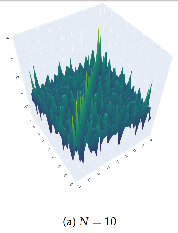
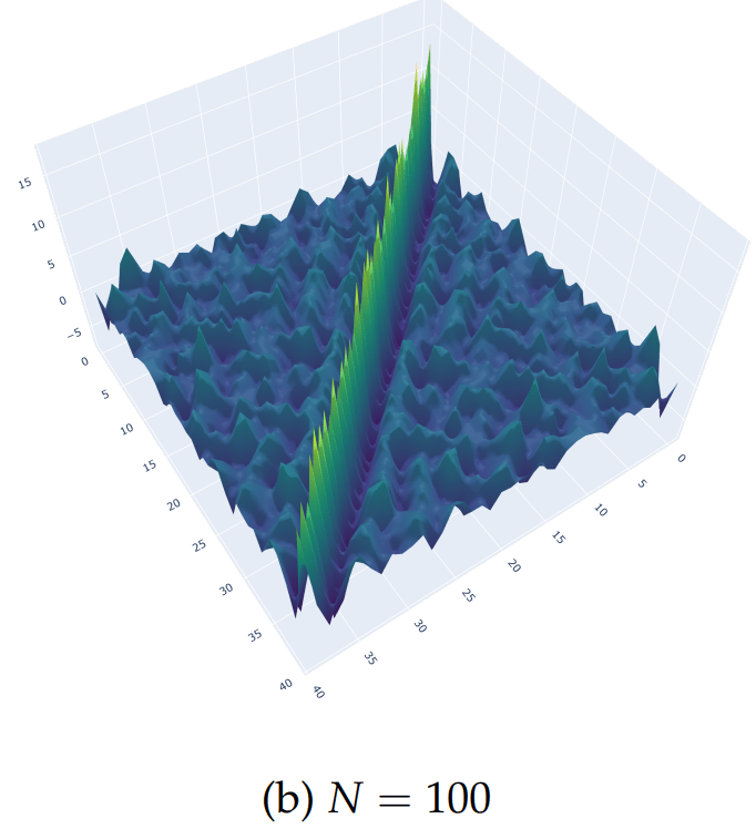
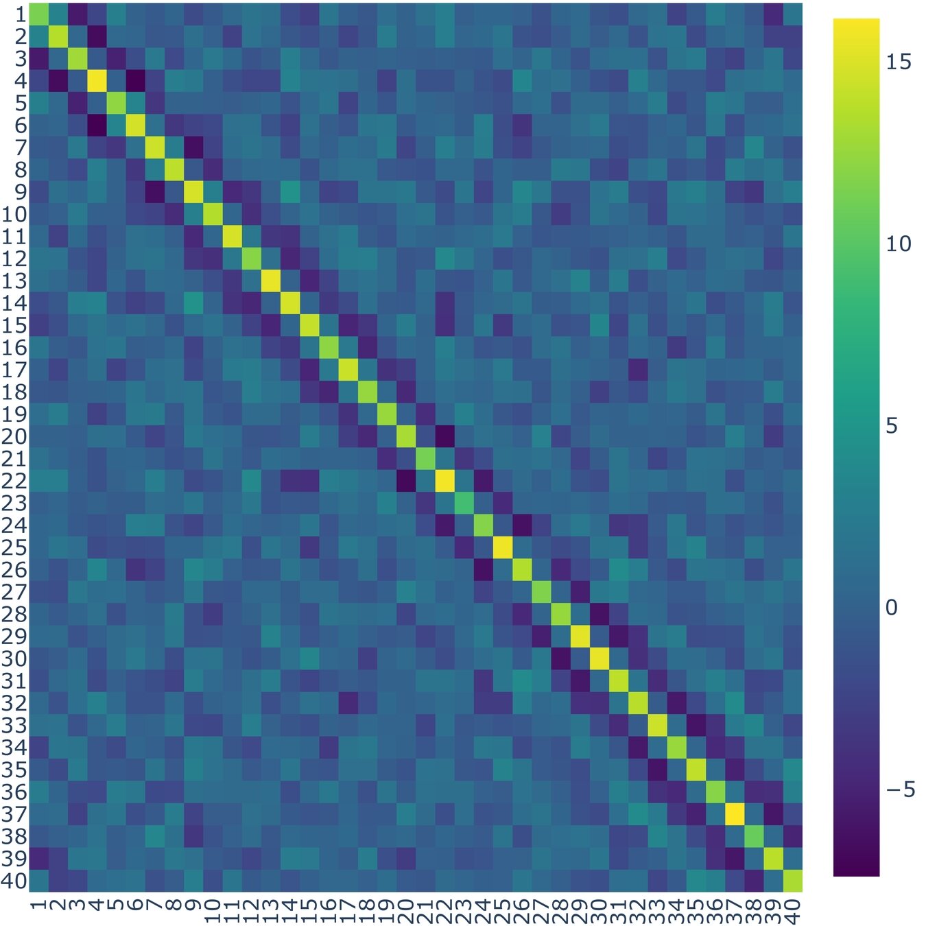
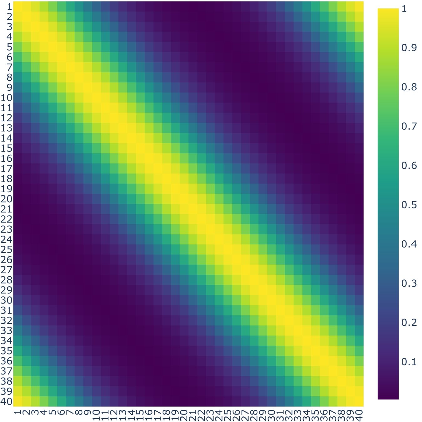
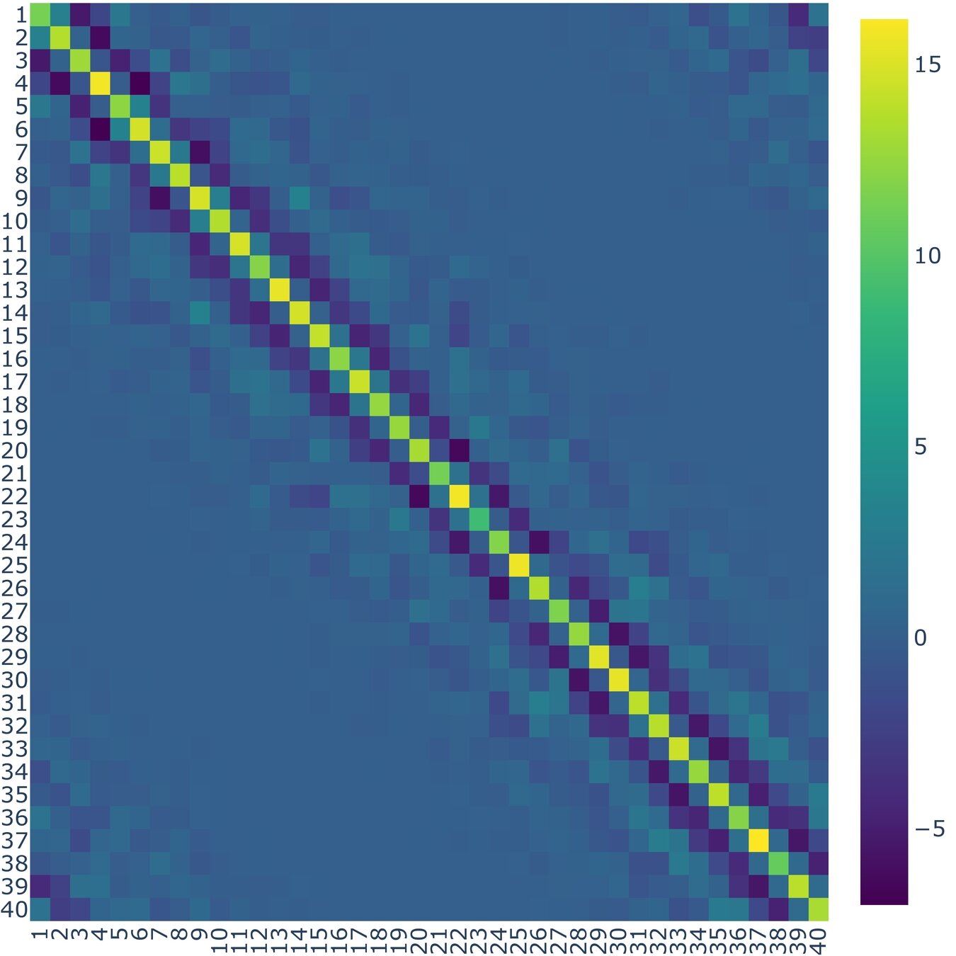
Localization Method
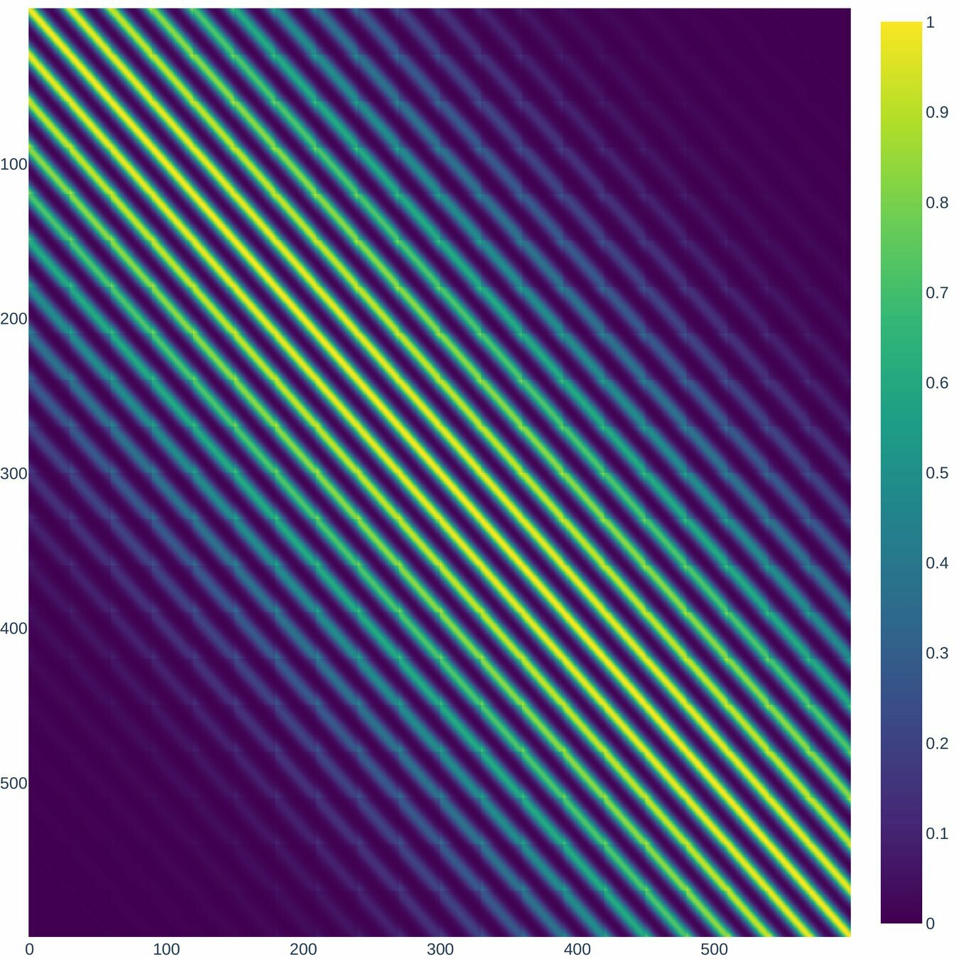
According to (Nino-Ruiz, 2021; Nino-Ruiz, Sandu, and Deng, 2018) in the context of covariance matrix localization, a decorrelation matrix is typically used in order to dissipate spurious correlations in spatially distant model components,
\Lambda \in \mathbb{R}^{n \times n}
\widehat{\mathbf{P}}^b = \Lambda \circ \mathbf{P}^{b} \in \mathbb{R}^{n \times n}
Where denotes the Schur product, is a localized covariance matrix, and the components of the localization matrix , for instance, reads
\circ
\widehat{\mathbf{P}}^b
\left(\Lambda\right)_{i,j} = \exp{\left[-\frac{1}{2} \cdot \frac{d\left(i,j\right)^{2}}{r^{2}}\right]}, \text{ For } 1 \leq i, j \leq n
\Lambda
Localization Method
\mathbf{P}^{b}
\mathbf{\Lambda}
Localization Method
\widehat{\mathbf{P}}^b = \Lambda \circ \mathbf{P}^{b} \in \mathbb{R}^{n \times n}
Proposed Method
General idea
The achievement of the mentioned objectives will be reflected in the construction of the following framework. It is worth mentioning that when creating Deep Learning models , these must undergo a training process, during which the parameters with which they are adjusted impact their learning and therefore their training.
\mathcal{M}
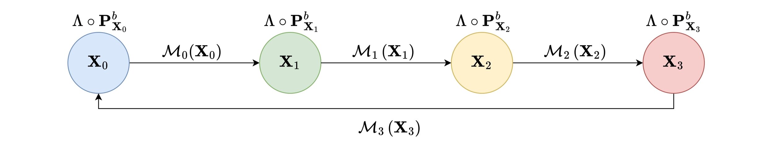
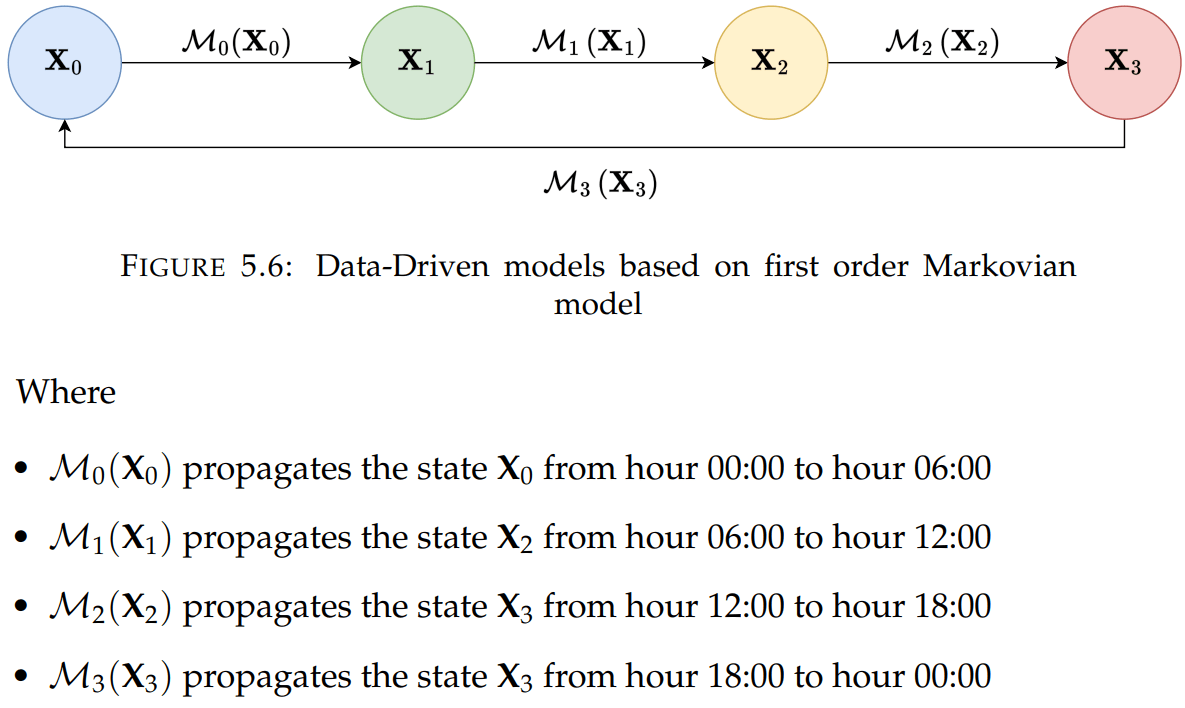
Scheme of Weather Forecasting based on First order Markovian model
Data

NetCDF Structure
Selected data
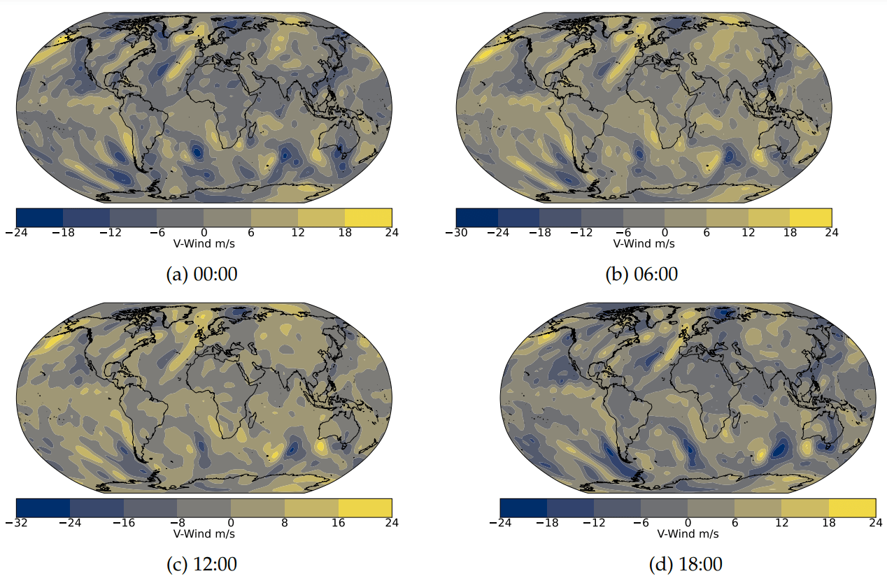
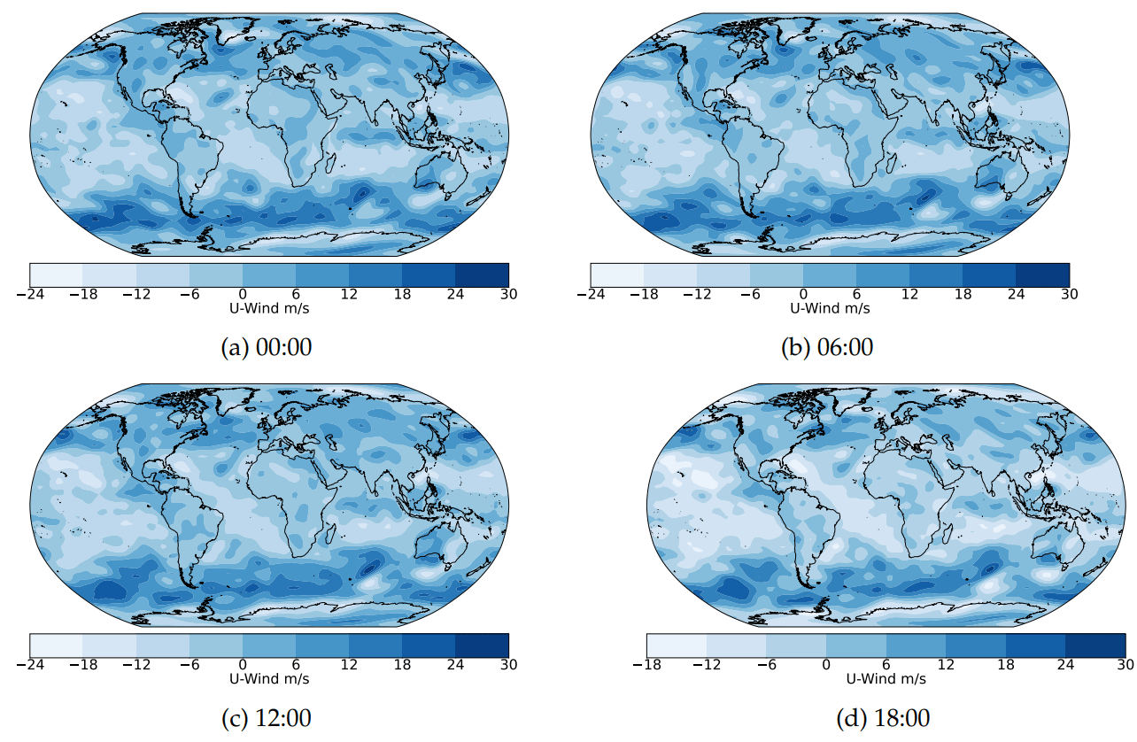
Weather variables include Air Temperature, U-Wind Component, and V-Wind Component, analyzed at the 1000hPa pressure level from 01-01-2020 00:00 to 31-12-2020 18:00. A global 2.5-degree latitude by 2.5-degree longitude grid (144x73) spanning 90N to 90S and 0E to 357.5E is used.
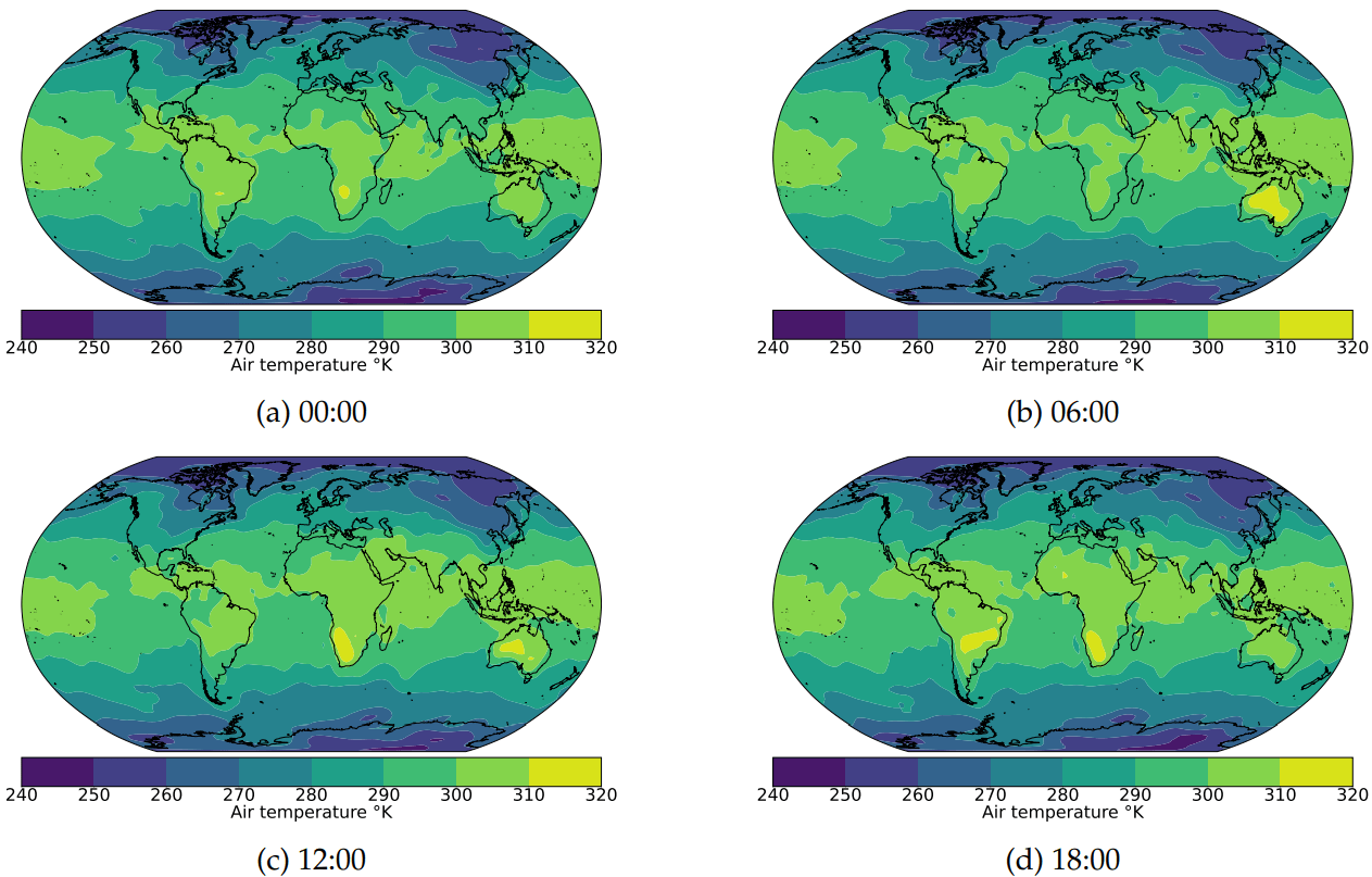
Air Temperature
U-Wind
V-Wind
Data - Driven model
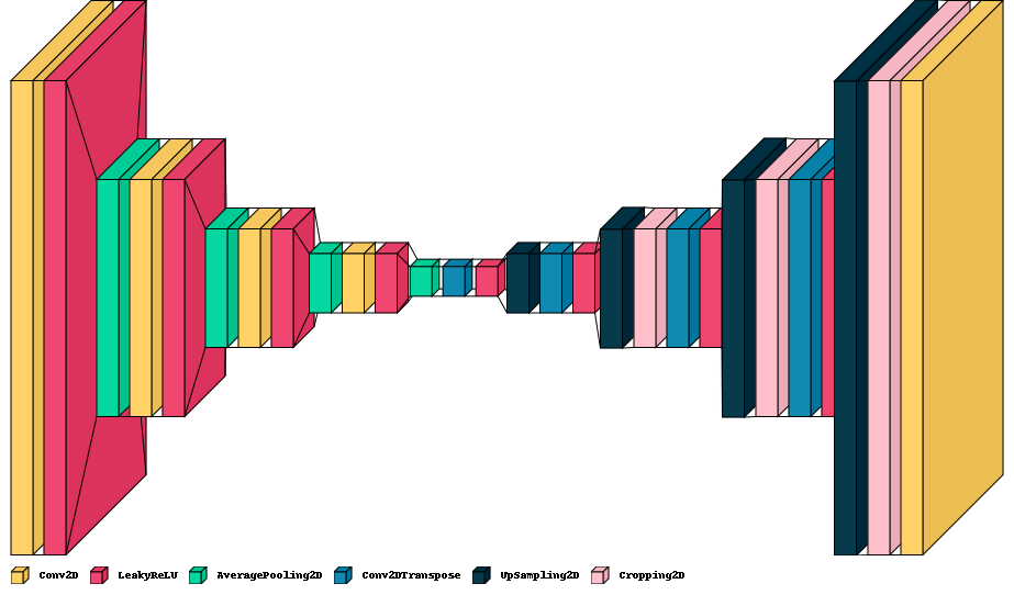
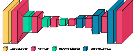
The architecture of the Data-Driven model is based on a convolutional autoencoder, as proposed by (Weyn et al., 2020), with some modifications, such as the activation function and cropping layer. This is necessary because the default framework used increases dimensions for even numbers. Additionally, a generic architecture can be observed for the trained transition models as follows:
Data - Driven Architecture
Training of Data - Driven model
During the training phase, it was considered training one model M for each study
variable at the aforementioned pressure level. This was done with the aim of generating the following transition scheme based on the predictions provided by each model
Hyperparameter optimization of the Data-driven model
is an open source hyperparameter optimization framework to automate
hyperparameter search (Akiba et al., 2019).
- Kernel size: This parameter refers to the size of the convolutional kernel used in the model, configurations considered: (2 × 2),(2 × 3),(2 × 4),(3 × 2),(3 × 3),(3 × 4),(4 × 2),(4 × 3),(4 × 4).
- Alpha for LeakyReLU function: Alpha is the slope of the negative region of the LeakyReLU activation function. It determines the rate at which the function leaks. Interval considered: [0.01, 0.9].
- Learning rate: This is the step size at which the model’s weights are updated during training. Interval considered: [0.0001, 0.01].
Results of optimizing models
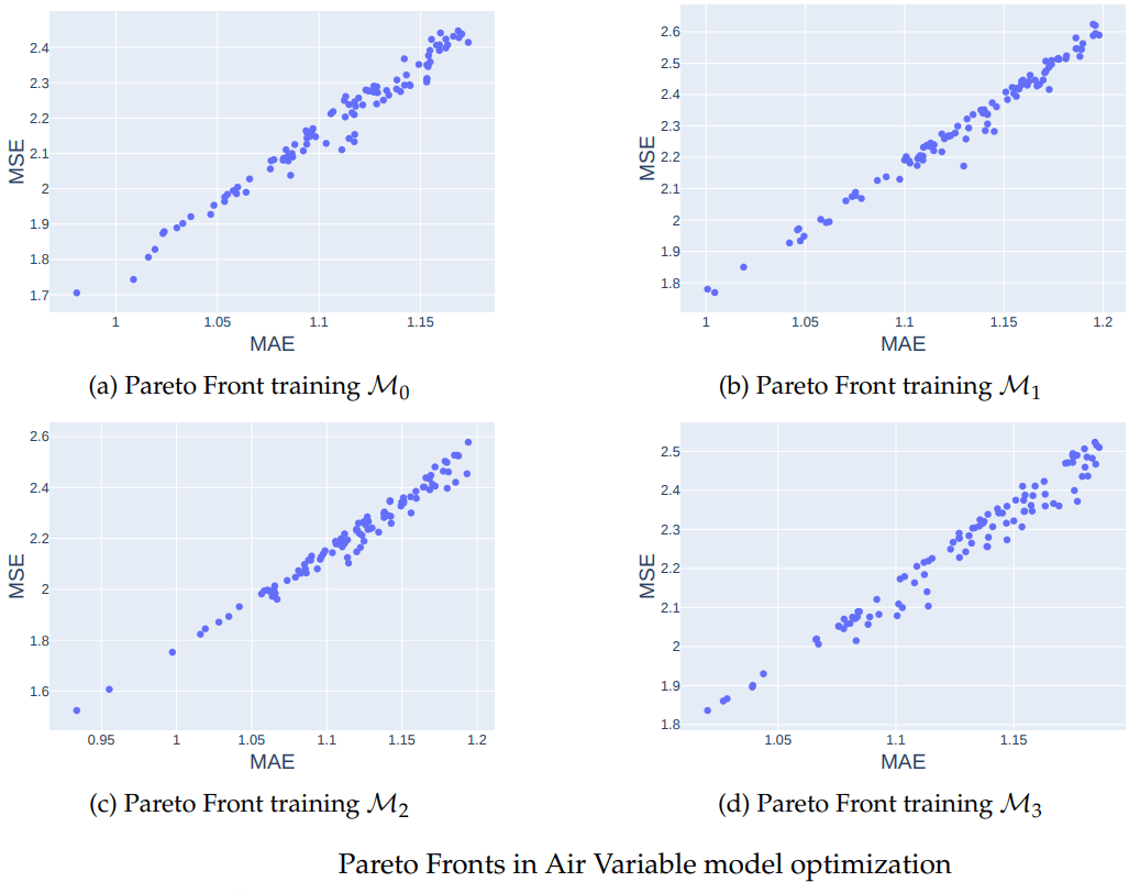
Results of optimizing models
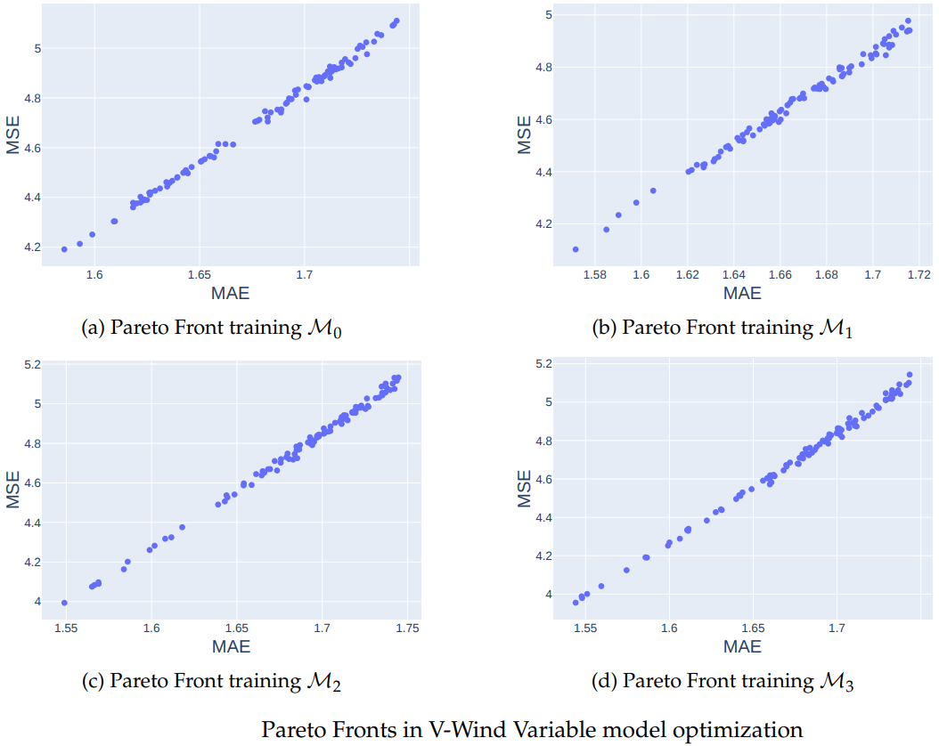
Results of optimizing models
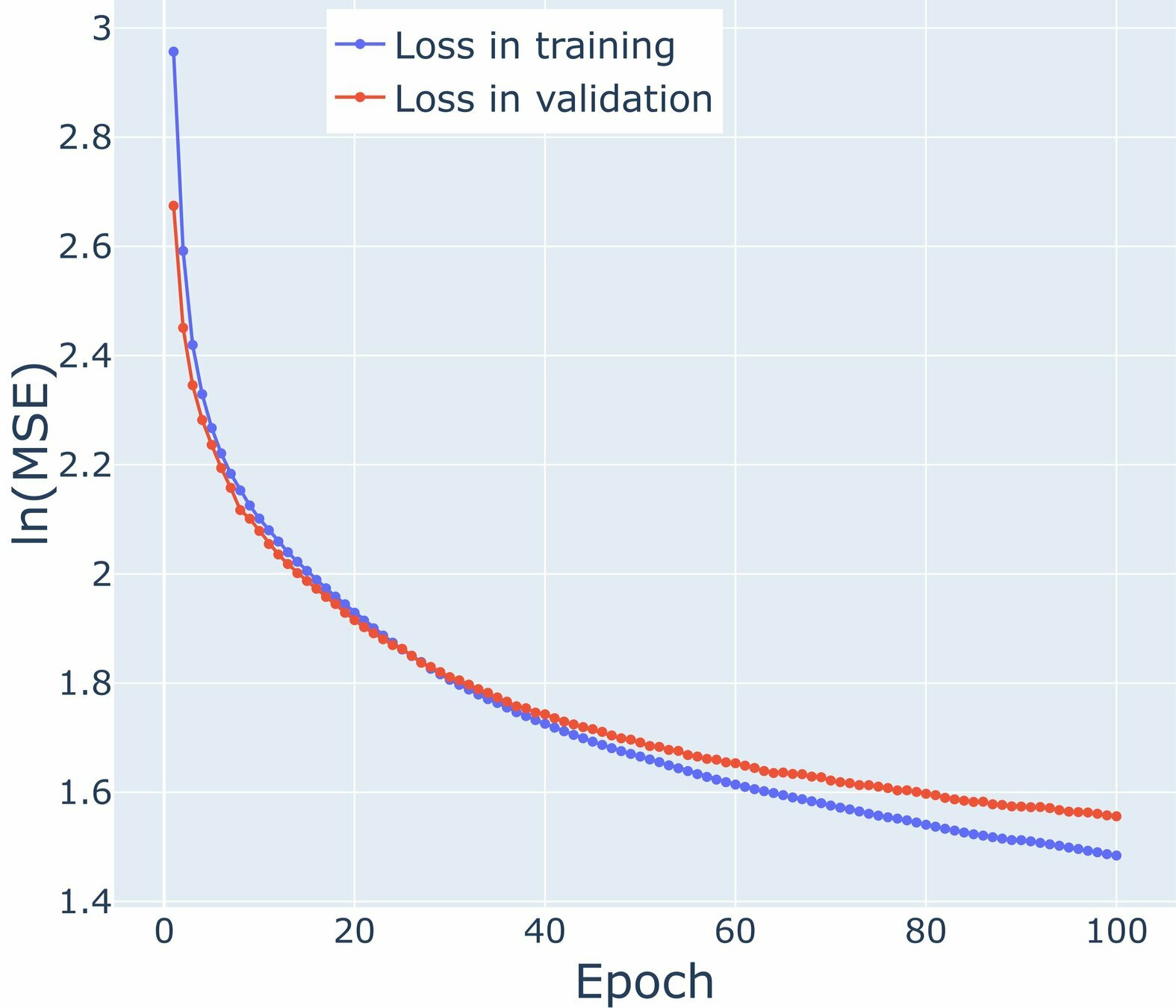
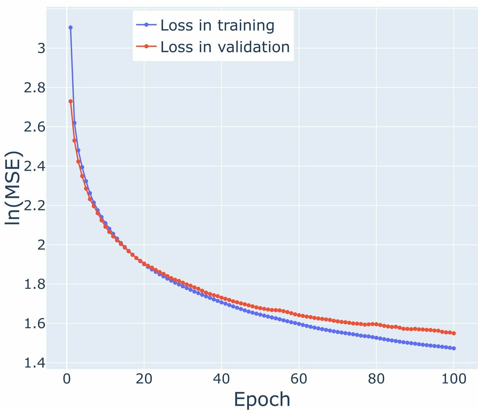
Loss graphs for Air Temperature

\mathcal{M}_0
\mathcal{M}_1
\mathcal{M}_2
\mathcal{M}_3
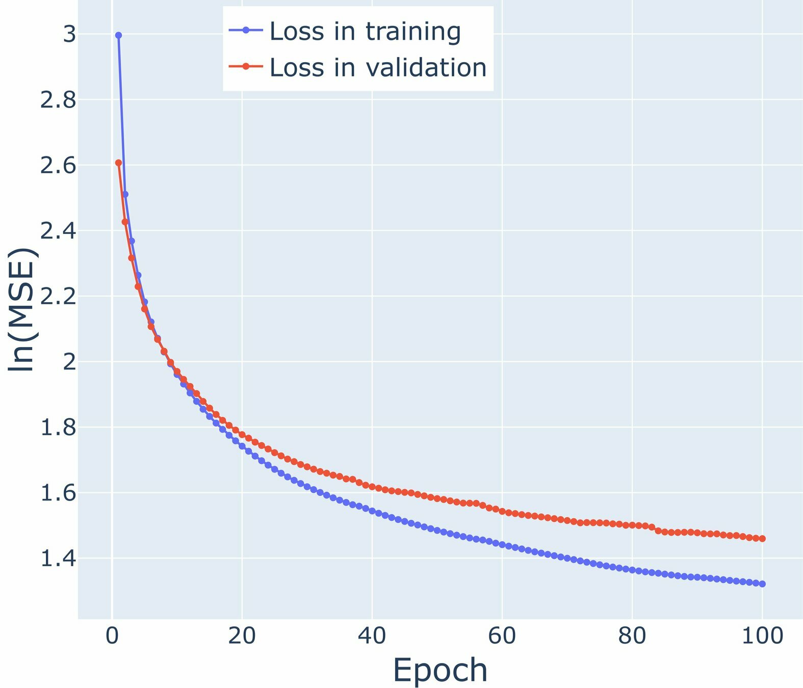
Loss graphs for V-Wind Component
\mathcal{M}_0
\mathcal{M}_1
\mathcal{M}_2
\mathcal{M}_3


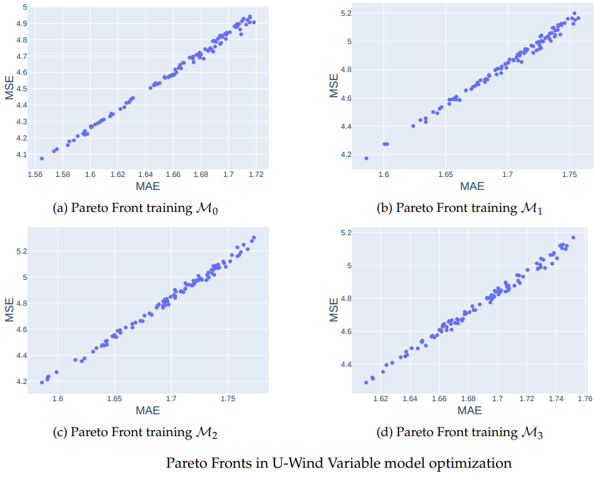
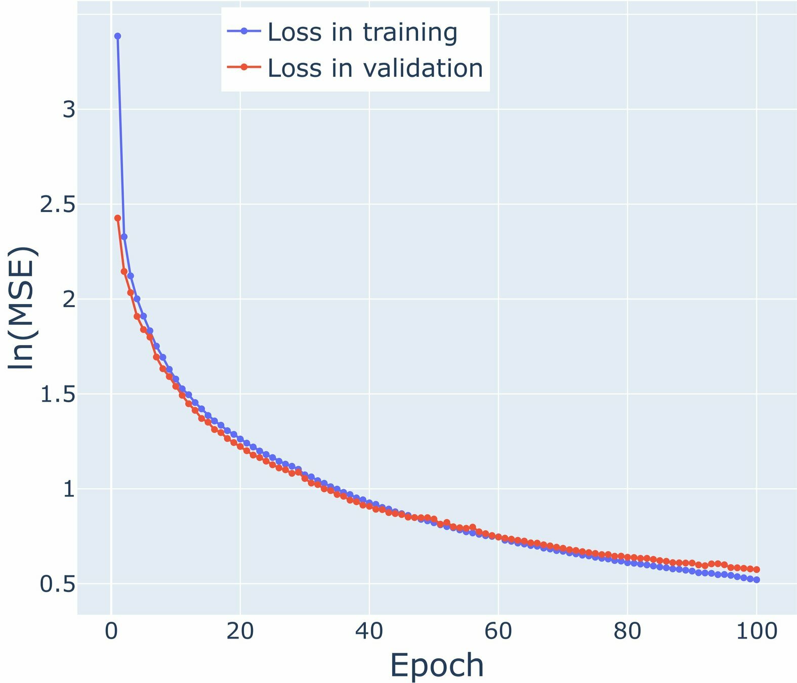
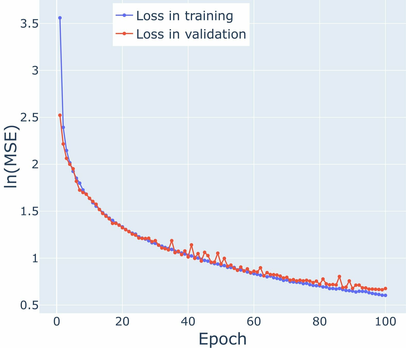
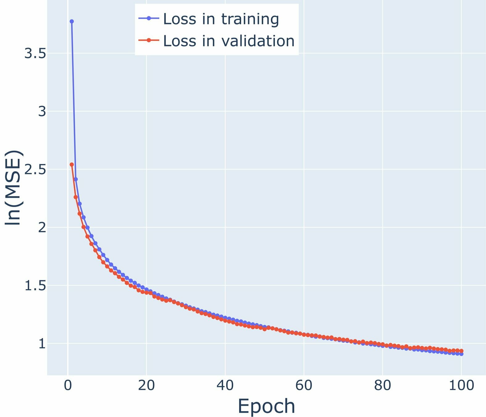
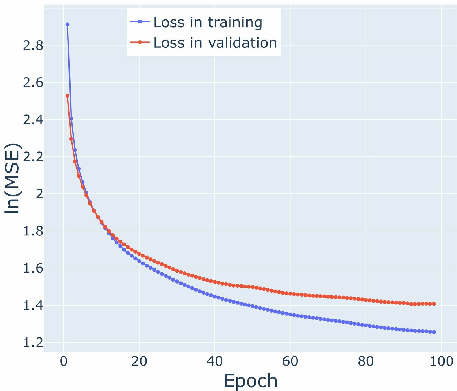
Train and Loss graphs for U-Wind Component
\mathcal{M}_0
\mathcal{M}_1
\mathcal{M}_2
\mathcal{M}_3

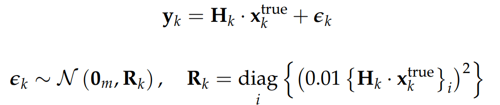
Localization Method for Ensemble Based on Data Assimilation
As mentioned before, the assimilation process, for instance, can be stochastically performed by:
Decorrelation matrix can be used to reduce the effects of sampling erros presented in the ensemble, recalling equation:

Localization Method for Ensemble Based on Data Assimilation
Therefore, it is possible to formulate the new way to perform the assimilation process as follows:
In this context, the assimilation process involves utilizing data from Reanalysis 2, wich will be presented in a 2-dimentional format. Consequently, the distance function is defined as the Euclidean distance:

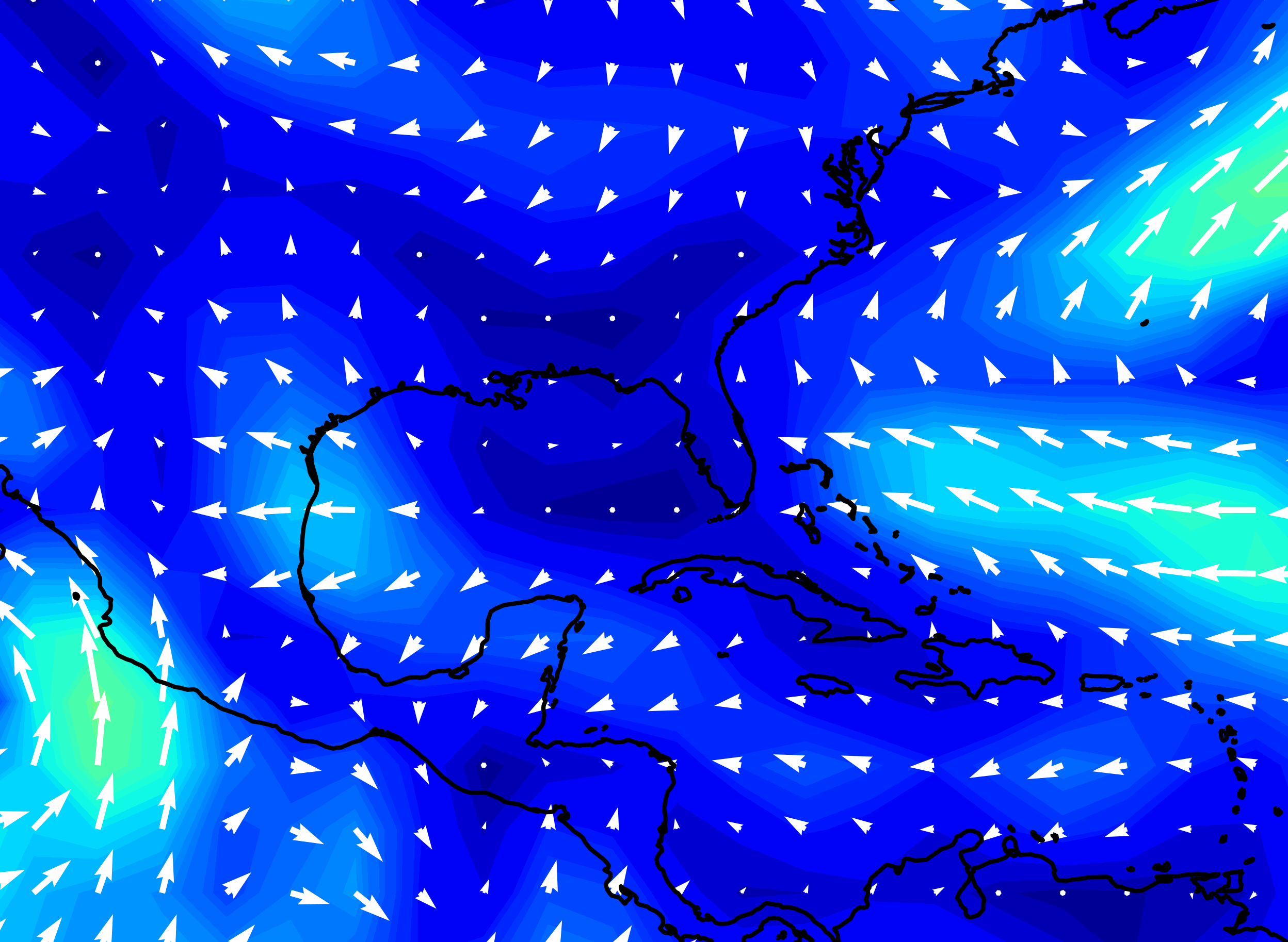
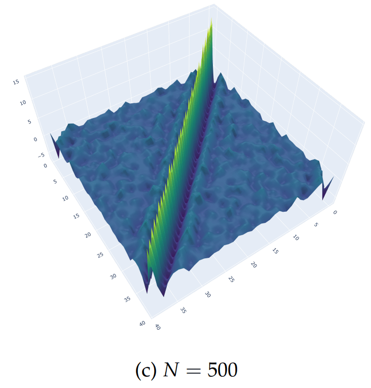
How is the Decorrelation matrix with the NOAA system dynamics?
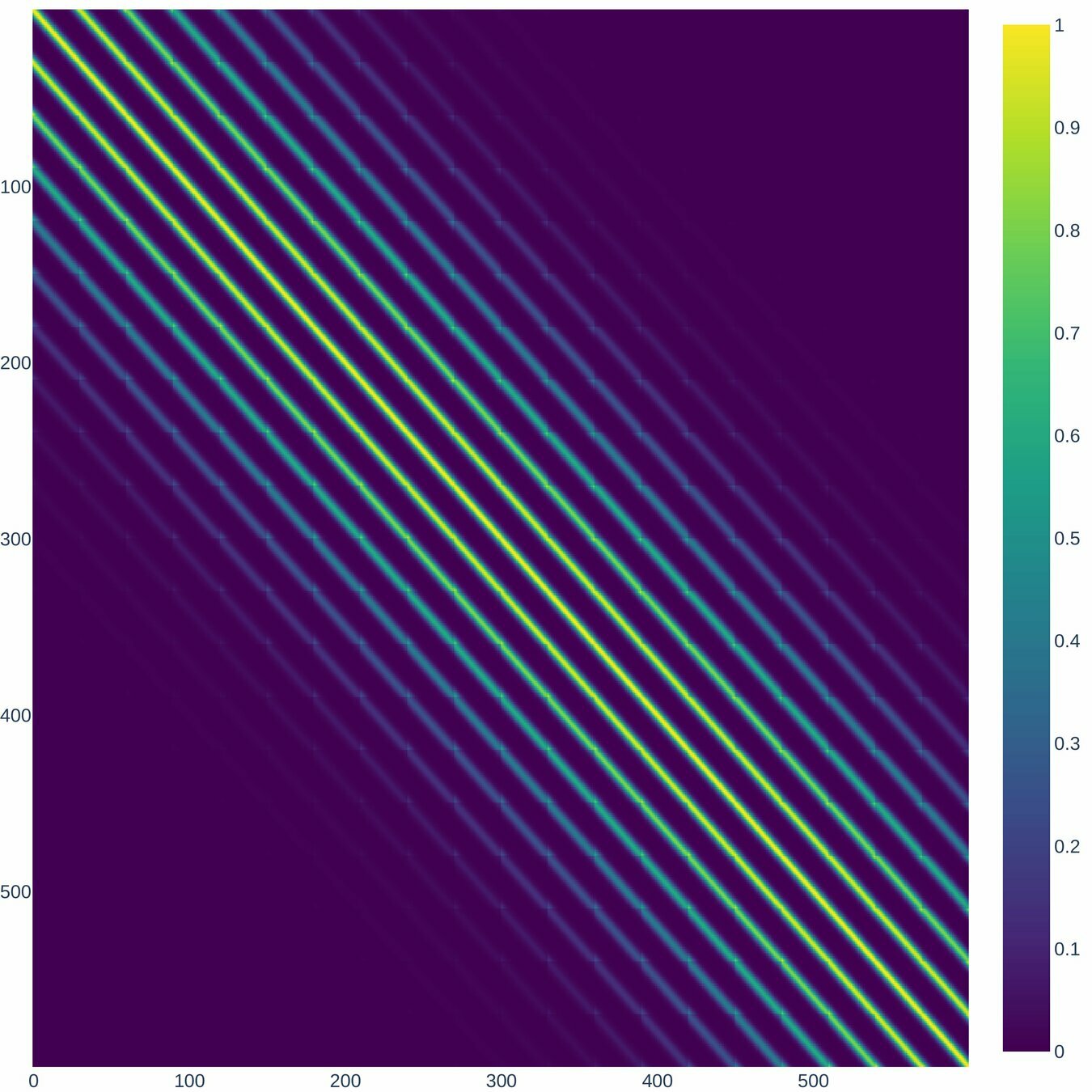
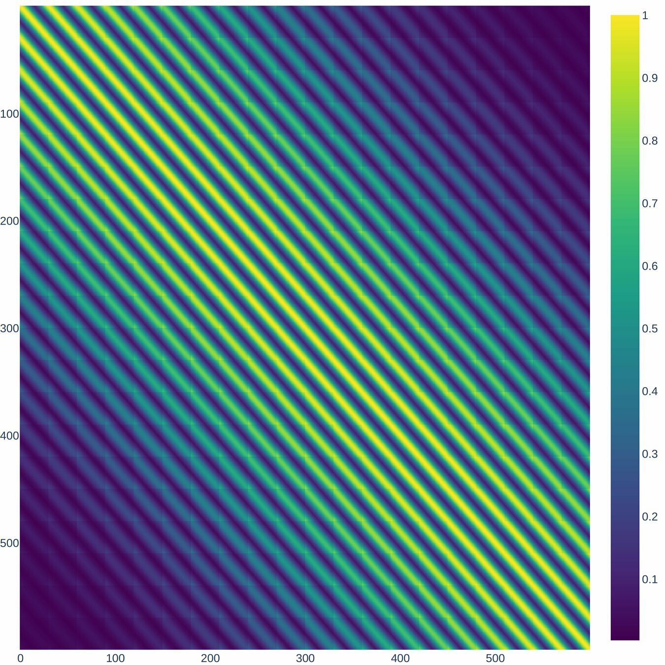
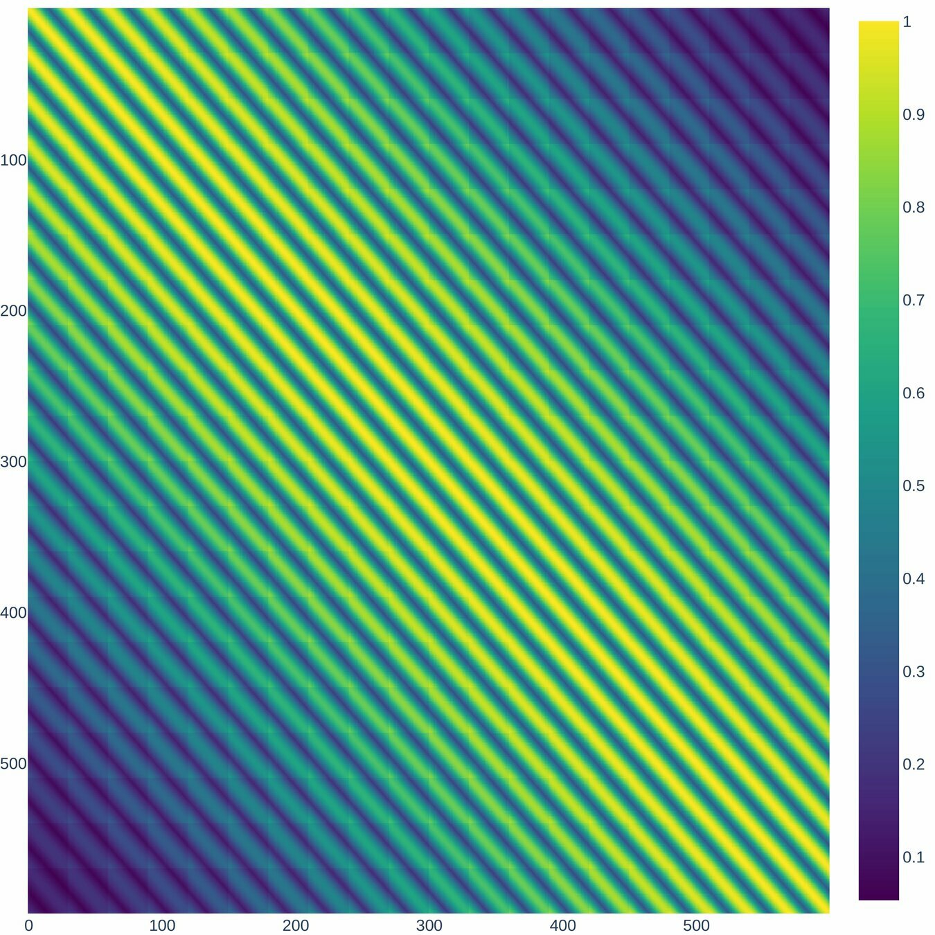
\Lambda, r=3
\Lambda, r=5
\Lambda, r=7
\Lambda, r=10
Numerical Experiments
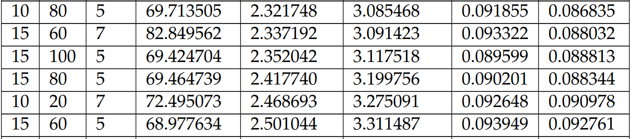
Parameters to run experiments
The testing period spans from November 1, 2023, to November 15, 2023, encompassing both the date of the initial ensemble creation and the subsequent trials
Note that the number of model components is n = 73 · 144 = 10512 and the maximum number of the ensemble members is N = 100 which means that N ≪ n, and the model space is approximately 106 times larger than the number of ensemble members.
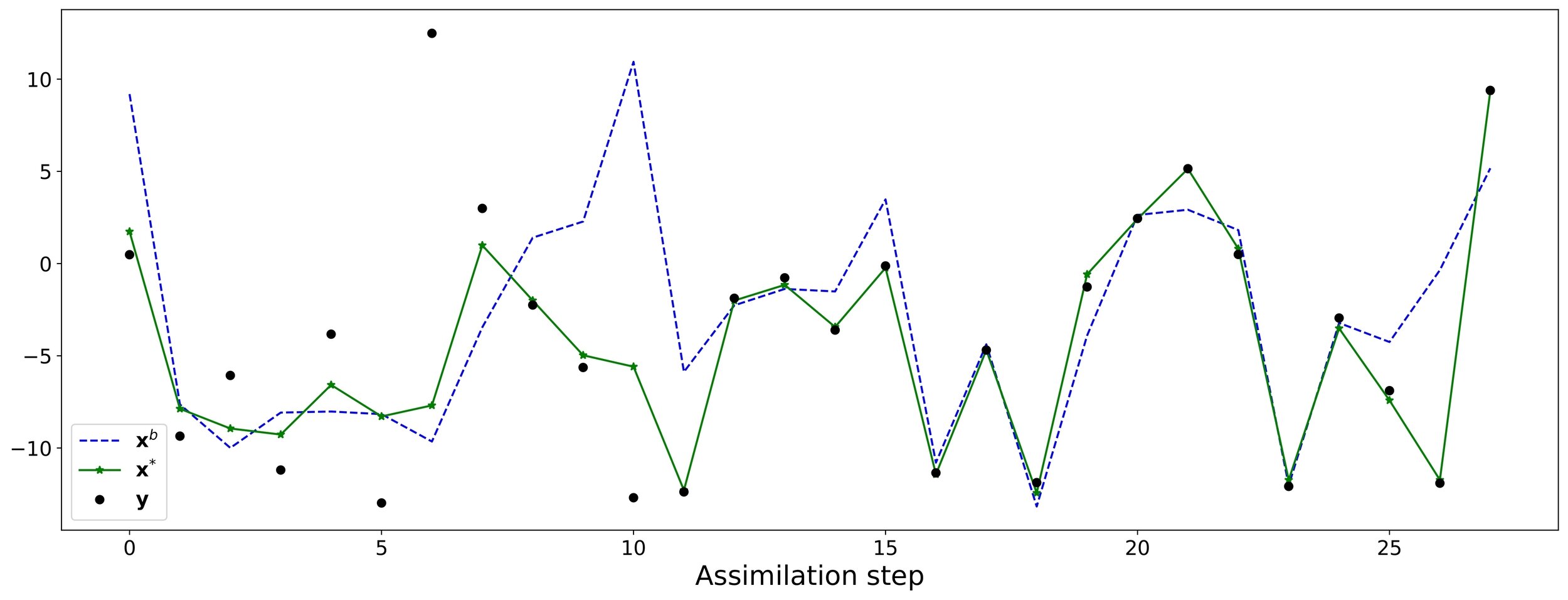
Initial Background and Observations
Initial ensemble is has the following structure


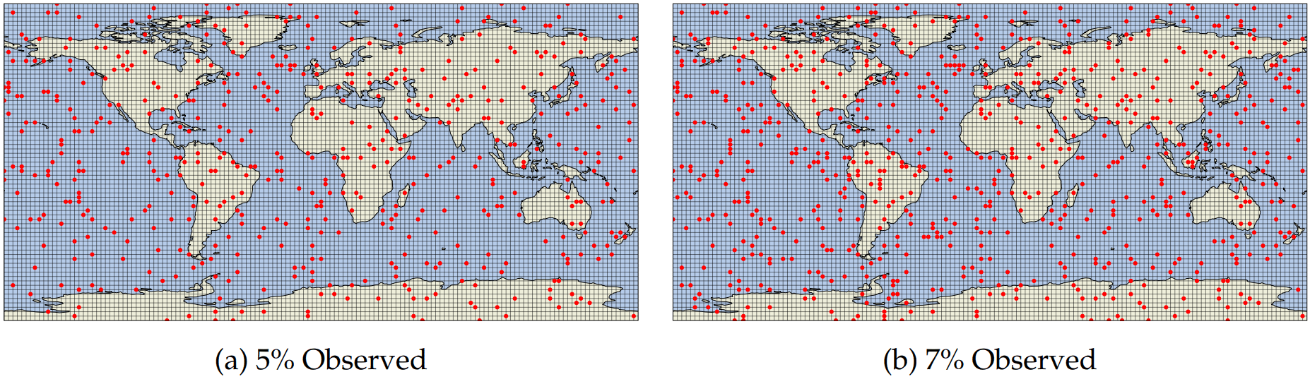
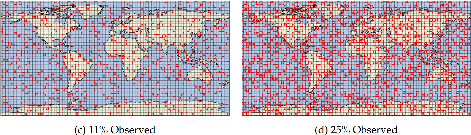
Observational networks
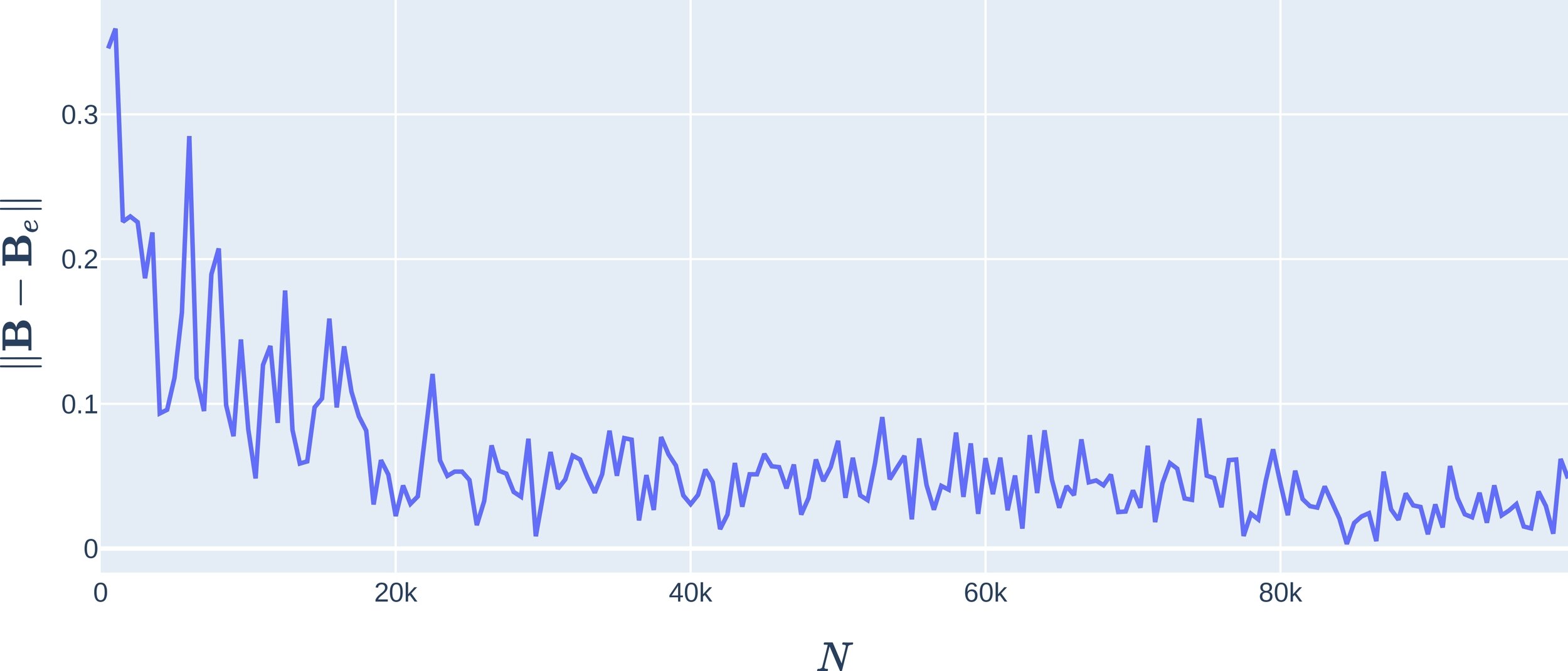
Metrics for analysis
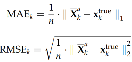
The precision of each analysis performed at time k is measured by the Mean Absolute Error and the Root Mean Squared Error
General Analysis for metrics

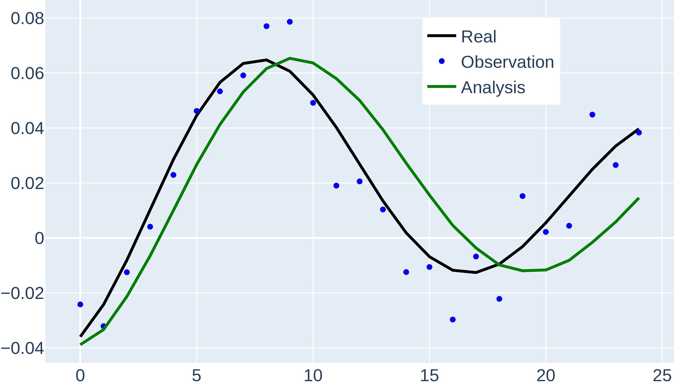
Snapshots for the best experiments
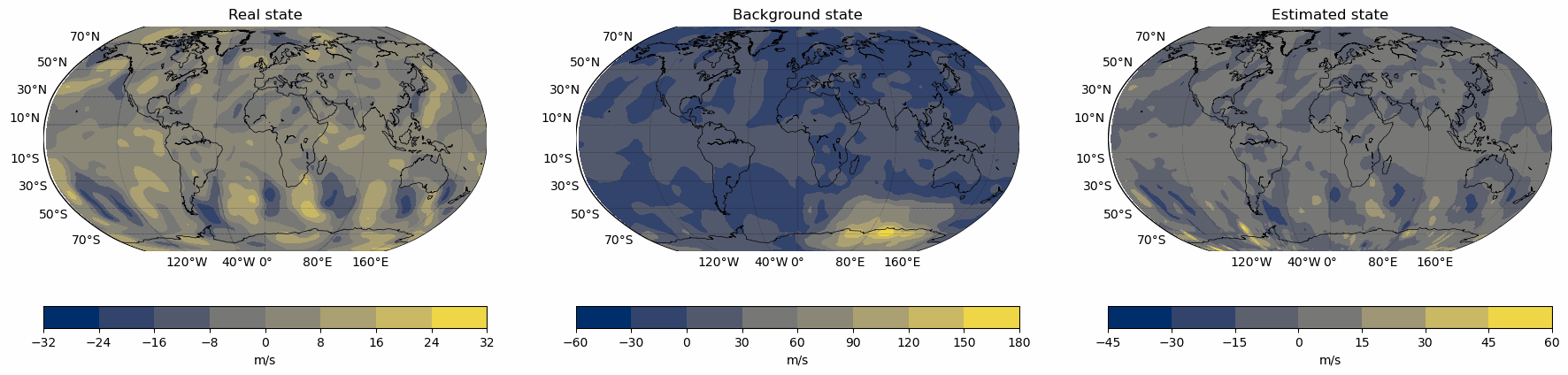
Air
Temperature
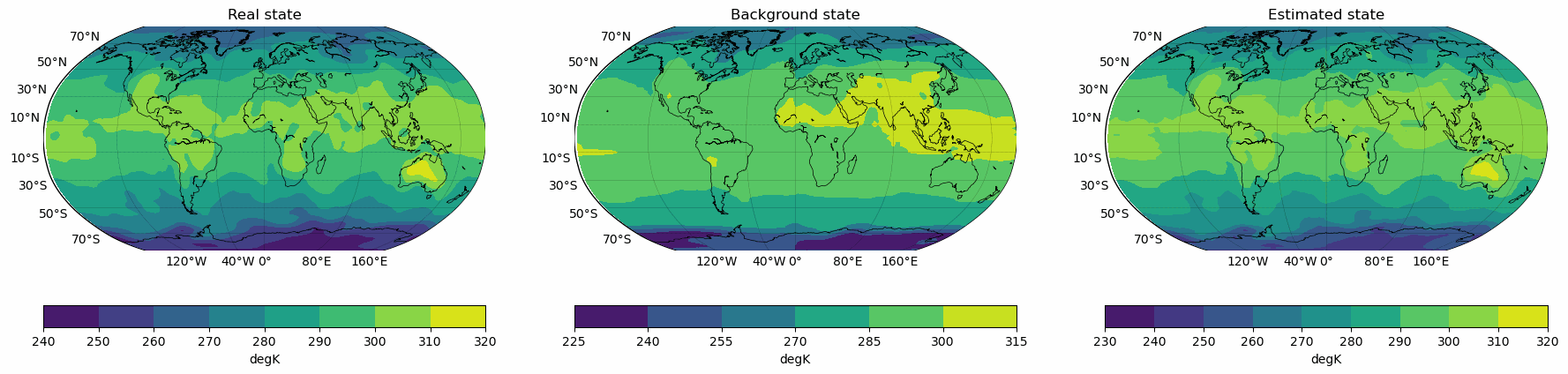
V-Wind
Component
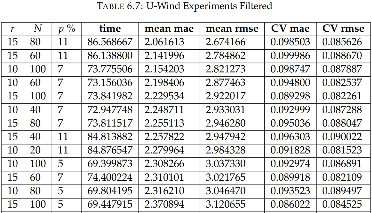
U-Wind
Component
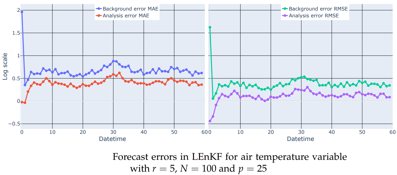
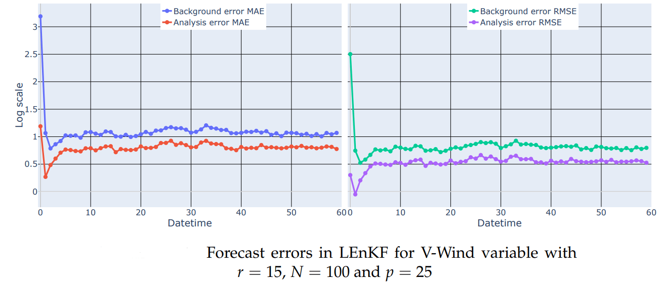
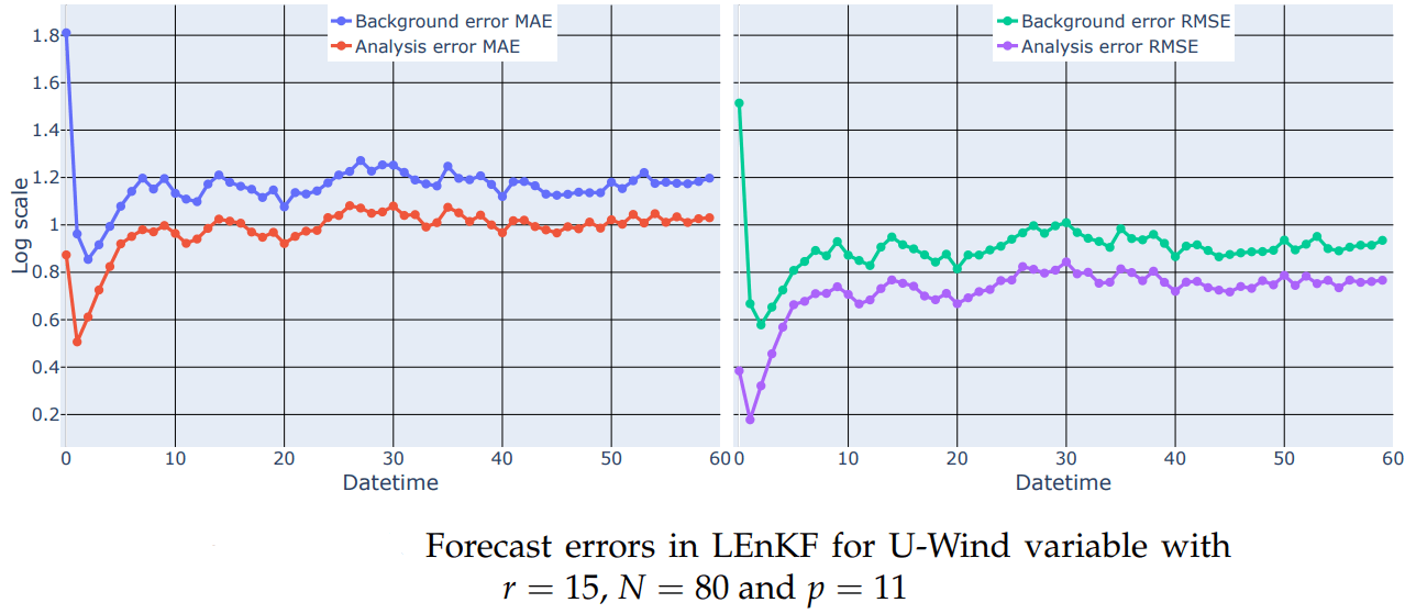
Erros for the best configuration
Erros for the best configuration
Erros for the best configuration
Conclusions
-
This master's thesis focuses on enhancing weather forecasting by implementing a model based on convolutional neural networks (CNNs) augmented with a data assimilation scheme.
-
The utilization of the Optuna framework has been instrumental in optimizing the hyperparameters of the transition model, thereby expanding the solution space effectively without imposing unnecessary constraints.
-
Our approach has demonstrated effectiveness in improving forecast accuracy, as evidenced by error metrics such as Mean Absolute Error (MAE) and Root Mean Square Error (RMSE).
-
Incorporating the decorrelation matrix into the formulation of the Local Ensemble Kalman Filter (LEnKF) has led to the reduction of spurious correlations, resulting in a more stable filter.
-
The stability of the filter has been validated through error evaluation metrics, thereby consolidating the effectiveness of the proposed methodology.
Future works
-
Exploration of additional data assimilation techniques is recommended, such as the application of the modified Cholesky method for estimating the inverse of the covariance matrix.
-
Consideration is suggested for other data-driven modeling techniques like Graph Neural Networks (GNNs) and Transformers, which could provide valuable insights into complex relationships in climatic patterns and enhance the modeling of long-term dependencies and scalability, respectively.
References
- Albawi, S., Mohammed, T. A., & Al-Zawi, S. (2017). Understanding of a convolu- tional neural network. 2017 international conference on engineering and technol- ogy (ICET), 1–6. https://doi.org/10.1109/ICEngTechnol.2017.8308186
- Anderson, J. L. (2001). An ensemble adjustment kalman filter for data assimilation. Monthly weather review, 129(12), 2884–2903. https://doi.org/10.1175/1520- 0493(2001)129%3C2884:AEAKFF%3E2.0.CO;2
- Asch, M., Bocquet, M., & Nodet, M. (2016). Data assimilation: Methods, algorithms, and applications. Society for Industrial; Applied Mathematics.
- Bishop, C. H., Etherton, B. J., & Majumdar, S. J. (2001). Adaptive sampling with the ensemble transform kalman filter. part i: Theoretical aspects. Monthly Weather Review, 129(3), 420–436. https://doi.org/https://doi.org/10.1175/1520- 0493(2001)129<0420:ASWTET>2.0.CO;2
- Burgers, G., Van Leeuwen, P. J., & Evensen, G. (1998). Analysis scheme in the ensem- ble kalman filter. Monthly weather review, 126(6), 1719–1724. https://doi.org/ 10.1175/1520-0493(1998)126%3C1719:ASITEK%3E2.0.CO;2
- Evensen, G. (1994). Sequential data assimilation with a nonlinear quasi-geostrophic model using monte carlo methods to forecast error statistics. Journal of Geo- physical Research: Oceans, 99(C5), 10143–10162.
- Evensen, G. (2003). The ensemble kalman filter: Theoretical formulation and practi- cal implementation. Ocean dynamics, 53, 343–367. https://doi.org/10.1007/ s10236-003-0036-9
- Evensen, G. (2006). Data assimilation: The ensemble kalman filter. Springer-Verlag.
- Fan, J., Liao, Y., & Liu, H. (2016). An overview of the estimation of large covariance and precision matrices. The Econometrics Journal, 19(1), C1–C32.
- Geron, A. (2019). Hands-on machine learning with scikit-learn, keras, and tensorflow: Con- cepts, tools, and techniques to build intelligent systems (2nd). O’Reilly Media, Inc.
- Gillijns, S., Mendoza, O., Chandrasekar, J., De Moor, B., Bernstein, D., & Ridley, A. (2006). What is the ensemble kalman filter and how well does it work? 2006 American Control Conference, 6 pp.-. https://doi.org/10.1109/ACC.2006.1657419
- Godinez, H. C., & Moulton, J. D. (2012). An efficient matrix-free algorithm for the ensemble kalman filter. Computational Geosciences, 16, 565–575. https://doi. org/10.1007/s10596-011-9268-9
- Golub, G. H., & Van Loan, C. F. (2013). Matrix computations. JHU press. Goodfellow, I., Bengio, Y., & Courville, A. (2016). Deep learning. The MIT Press.
- Houtekamer, P. L., & Mitchell, H. L. (1998). Data assimilation using an ensemble kalman filter technique. Monthly Weather Review, 126(3), 796–811. https:// doi.org/10.1175/1520-0493(1998)126%3C0796:DAUAEK%3E2.0.CO;2
- Jaseena, K. U., & Kovoor, B. C. (2022). Deterministic weather forecasting models based on intelligent predictors: A survey. JOURNAL OF KING SAUD UNIVERSITY- COMPUTER AND INFORMATION SCIENCES, 34(6, B), 3393–3412. https://doi.org/10.1016/j.jksuci.2020.09.009
- Kalman, R. E., & Bucy, R. S. (1961). New results in linear filtering and prediction theory.
- Kalman, R. E. (1960). A new approach to linear filtering and prediction problems.
- Kalnay, E. (2003). Atmospheric modeling, data assimilation and predictability. Cambridge university press.
- Kanamitsu, M., Ebisuzaki, W., Woollen, J., Yang, S.-K., Hnilo, J. J., Fiorino, M., & Potter, G. L. (2002). Ncep–doe amip-ii reanalysis (r-2). Bulletin of the American Meteorological Society, 83(11), 1631–1644. https://doi.org/https://doi.org/ 10.1175/BAMS-83-11-1631
- Karevan, Z., & Suykens, J. A. K. (2020). Transductive lstm for time-series predic- tion: An application to weather forecasting. NEURAL NETWORKS, 125, 1–9. https://doi.org/10.1016/j.neunet.2019.12.030
- Lahoz, W., Boris, K., & Ménard, R. (2010). Data assimilation. Springer.
- Liu, N., & Oliver, D. S. (2005, January). Critical Evaluation of the Ensemble Kalman Filter on History Matching of Geologic Facies (Vol. All Days). https://doi.org/ 10.2118/92867-MS
- Lorenc, A. C. (2003). The potential of the ensemble kalman filter for nwp—a com- parison with 4d-var. Quarterly Journal of the Royal Meteorological Society: A journal of the atmospheric sciences, applied meteorology and physical oceanography, 129(595), 3183–3203.
- McLaughlin, D. (2014). Data assimilation. In E. G. Njoku (Ed.), Encyclopedia of remote sensing (pp. 131–134). Springer New York. https://doi.org/10.1007/978-0- 387-36699-9_33
- Ng, A., et al. (2011). Sparse autoencoder. CS294A Lecture notes, 72(2011), 1–19.
- Nino Ruiz, E. D., Sandu, A., & Anderson, J. (2015). An efficient implementation of the ensemble kalman filter based on an iterative sherman–morrison formula. Statistics and Computing, 25, 561–577. https://doi.org/10.1016/j.procs.2012.04.115
- Nino-Ruiz, E. D. (2021). A data-driven localization method for ensemble based data assimilation. Journal of Computational Science, 51, 101328. https://doi.org/ https://doi.org/10.1016/j.jocs.2021.101328
- Nino-Ruiz, E. D., Mancilla, A., & Calabria, J. C. (2017). A posterior ensemble kalman filter based on a modified cholesky decomposition [International Conference on Computational Science, ICCS 2017, 12-14 June 2017, Zurich, Switzerland]. Procedia Computer Science, 108, 2049–2058. https://doi.org/https://doi.org/ 10.1016/j.procs.2017.05.062
- Nino-Ruiz, E. D., Sandu, A., & Deng, X. (2018). An ensemble kalman filter imple- mentation based on modified cholesky decomposition for inverse covariance matrix estimation. SIAM Journal on Scientific Computing, 40(2), A867–A886. https://doi.org/10.1137/16M1097031
- Pourahmadi, M. (2011). Covariance Estimation: The GLM and Regularization Per- spectives. Statistical Science, 26(3), 369–387. https://doi.org/10.1214/11- STS358
- Rasp, S., Dueben, P. D., Scher, S., Weyn, J. A., Mouatadid, S., & Thuerey, N. (2020). Weatherbench: A benchmark data set for data-driven weather forecasting [e2020MS002203 10.1029/2020MS002203]. Journal of Advances in Modeling Earth Systems, 12(11), e2020MS002203. https://doi.org/https://doi.org/10.1029/ 2020MS002203
- Salman, A. G., Kanigoro, B., & Heryadi, Y. (2015). Weather forecasting using deep learning techniques. 2015 International Conference on Advanced Computer Sci- ence and Information Systems (ICACSIS), 281–285. https://doi.org/10.1109/ ICACSIS.2015.7415154
- Samuel, A. L. (1959). Some studies in machine learning using the game of checkers. IBM Journal of Research and Development, 3(3), 210–229. https://doi.org/10. 1147/rd.33.0210
- Sun, M., Song, Z., Jiang, X., Pan, J., & Pang, Y. (2017). Learning pooling for convo- lutional neural network. Neurocomputing, 224, 96–104. https://doi.org/10. 1016/j.neucom.2016.10.049
- Tandeo, P., Ailliot, P., Bocquet, M., Carrassi, A., Miyoshi, T., Pulido, M., & Zhen, Y. (2018). Joint estimation of model and observation error covariance matrices in data assimilation: A review.
- Vetra-Carvalho, S., Van Leeuwen, P. J., Nerger, L., Barth, A., Altaf, M. U., Brasseur, P., Kirchgessner, P., & Beckers, J.-M. (2018). State-of-the-art stochastic data assimilation methods for high-dimensional non-gaussian problems. Tellus A: Dynamic Meteorology and Oceanography, 70(1), 1–43.
- Wang, X., Hamill, T. M., Whitaker, J. S., & Bishop, C. H. (2007). A comparison of hy- brid ensemble transform kalman filter–optimum interpolation and ensemble square root filter analysis schemes. Monthly weather review, 135(3), 1055–1076. https://doi.org/10.1175/MWR3307.1
- Weyn, J. A., Durran, D. R., & Caruana, R. (2020). Improving data-driven global weather prediction using deep convolutional neural networks on a cubed sphere. Journal of Advances in Modeling Earth Systems, 12(9), e2020MS002109. https://doi.org/10.1029/2020MS002109
- Woodbury, M. A. (1950). Inverting modified matrices. Department of Statistics, Prince- ton University.
Thesis
By Sebastian Ariza


