

Lecture 11: Reinforcement Learning
Shen Shen
April 25, 2025
11am, Room 10-250
Intro to Machine Learning

Outline
- Recap: Markov decision processes
- Reinforcement learning setup
- Model-based methods
- Model-free methods
- (tabular) Q-learning
- \(\epsilon\)-greedy action selection
- exploration vs. exploitation
- (neural network) Q-learning
- (tabular) Q-learning
- Reinforcement learning setup again
- \(\mathcal{S}\) : state space, contains all possible states \(s\).
- \(\mathcal{A}\) : action space, contains all possible actions \(a\).
- \(\mathrm{T}\left(s, a, s^{\prime}\right)\) : the probability of transition from state \(s\) to \(s^{\prime}\) when action \(a\) is taken.
- \(\mathrm{R}(s, a)\) : reward, takes in a (state, action) pair and returns a reward.
- \(\gamma \in [0,1]\): discount factor, a scalar.
- \(\pi{(s)}\) : policy, takes in a state and returns an action.
The goal of an MDP is to find a "good" policy.
Markov Decision Processes - Definition and terminologies
In 6.390,
- \(\mathcal{S}\) and \(\mathcal{A}\) are small discrete sets, unless otherwise specified.
- \(s^{\prime}\) and \(a^{\prime}\) are short-hand for the next-timestep
- \(\mathrm{R}(s, a)\) is deterministic and bounded.
- \(\pi(s)\) is deterministic.
\mathrm{V}_h^\pi(s)=\mathrm{R}\left(s, \pi(s)\right)+\gamma \sum_{s^{\prime}} \mathrm{T}\left(s, \pi(s), s^{\prime}\right) \mathrm{V}_{h-1}^\pi\left(s^{\prime}\right)
the immediate reward for taking the policy-prescribed action \(\pi(s)\) in state \(s\).
horizon-\(h\) value in state \(s\): the expected sum of discounted rewards, starting in state \(s\) and following policy \(\pi\) for \(h\) steps.
\((h-1)\) horizon future values at a next state \(s^{\prime}\)
sum up future values weighted by the probability of getting to that next state \(s^{\prime}\)
discounted by \(\gamma\)
finite-horizon Bellman recursions
infinite-horizon Bellman equations
\mathrm{V}^\pi_{\infty}(s)= \mathrm{R}(s, \pi(s))+ \gamma \sum_{s^{\prime}} \mathrm{T}\left(s, \pi(s), s^{\prime}\right) \mathrm{V}^\pi_{\infty}\left(s^{\prime}\right), \forall s
\mathrm{V}_{h}^\pi(s)= \mathrm{R}(s, \pi(s))+ \gamma \sum_{s^{\prime}} \mathrm{T}\left(s, \pi(s), s^{\prime}\right) \mathrm{V}_{h-1}^\pi\left(s^{\prime}\right), \forall s
Recall: For a given policy \(\pi(s),\) the (state) value functions
\(\mathrm{V}_h^\pi(s):=\mathbb{E}\left[\sum_{t=0}^{h-1} \gamma^t \mathrm{R}\left(s_t, \pi\left(s_t\right)\right) \mid s_0=s, \pi\right], \forall s, h\)
\pi(s)
\mathrm{V}^{\pi}_{h}(s)
MDP
Policy evaluation
1. By summing \(h\) terms:
2. By leveraging structure:
Given the recursion
\mathrm{Q}^*_{\infty}(s, a)=\mathrm{R}(s, a)+\gamma \sum_{s^{\prime}} \mathrm{T}\left(s, a, s^{\prime} \right) \max _{a^{\prime}} \mathrm{Q}^*_{\infty}\left(s^{\prime}, a^{\prime}\right)
- for \(s \in \mathcal{S}, a \in \mathcal{A}\) :
- \(\mathrm{Q}_{\text {old }}(\mathrm{s}, \mathrm{a})=0\)
- while True:
- for \(s \in \mathcal{S}, a \in \mathcal{A}\) :
- \(\mathrm{Q}_{\text {new }}(s, a) \leftarrow \mathrm{R}(s, a)+\gamma \sum_{s^{\prime}} \mathrm{T}\left(s, a, s^{\prime}\right) \max _{a^{\prime}} \mathrm{Q}_{\text {old }}\left(s^{\prime}, a^{\prime}\right)\)
- if \(\max _{s, a}\left|Q_{\text {old }}(s, a)-Q_{\text {new }}(s, a)\right|<\epsilon:\)
- return \(\mathrm{Q}_{\text {new }}\)
- \(\mathrm{Q}_{\text {old }} \leftarrow \mathrm{Q}_{\text {new }}\)
\mathrm{Q}^*_h (s, a)=\mathrm{R}(s, a)+\gamma \sum_{s^{\prime}} \mathrm{T}\left(s, a, s^{\prime} \right) \max _{a^{\prime}} \mathrm{Q}^*_{h-1}\left(s^{\prime}, a^{\prime}\right)
we can have an infinite-horizon equation
Value Iteration
if run this block \(h\) times and break, then the returns are exactly \(\mathrm{Q}^*_h\)
\{
\(\mathrm{Q}^*_{\infty}(s, a)\)
Outline
- Recap: Markov decision processes
- Reinforcement learning setup
- Model-based methods
- Model-free methods
- (tabular) Q-learning
- \(\epsilon\)-greedy action selection
- exploration vs. exploitation
- (neural network) Q-learning
- (tabular) Q-learning
- Reinforcement learning setup again
- (state, action) results in a transition into a next state:
-
Normally, we get to the “intended” state;
-
E.g., in state (7), action “↑” gets to state (4)
-
-
If an action would take Mario out of the grid world, stay put;
-
E.g., in state (9), “→” gets back to state (9)
-
-
In state (6), action “↑” leads to two possibilities:
-
20% chance to (2)
-
80% chance to (3)
-
-
80\%
20\%
Running example: Mario in a grid-world

- 9 possible states
- 4 possible actions: {Up ↑, Down ↓, Left ←, Right →}
1
2
9
8
7
5
4
3
6
Recall
1
1
1
1
-10
-10
-10
-10
reward of (3, \(\downarrow\))
reward of \((3,\uparrow\))
reward of \((6, \downarrow\))
reward of \((6,\rightarrow\))
- (state, action) pairs give out rewards:
- in state 3, any action gives reward 1
- in state 6, any action gives reward -10
- any other (state, action) pair gives reward 0
-
discount factor: a scalar of 0.9 that reduces the "worth" of rewards, depending on the timing we receive them.
- e.g., for (3, \(\leftarrow\)) pair, we receive a reward of 1 at the start of the game; at the 2nd time step, we receive a discounted reward of 0.9; at the 3rd time step, it is further discounted to \((0.9)^2\), and so on.

Mario in a grid-world, cont'd
- transition probabilities are unknown
Running example: Mario in a grid-world
Reinforcement learning setup
- 9 possible states
- 4 possible actions: {Up ↑, Down ↓, Left ←, Right →}
- rewards unknown
- discount factor \(\gamma = 0.9\)
Now

?
?
?
\dots
?

- \(\mathcal{S}\) : state space, contains all possible states \(s\).
- \(\mathcal{A}\) : action space, contains all possible actions \(a\).
- \(\mathrm{T}\left(s, a, s^{\prime}\right)\) : the probability of transition from state \(s\) to \(s^{\prime}\) when action \(a\) is taken.
- \(\mathrm{R}(s, a)\) : reward, takes in a (state, action) pair and returns a reward.
- \(\gamma \in [0,1]\): discount factor, a scalar.
- \(\pi{(s)}\) : policy, takes in a state and returns an action.
The goal of an MDP problem is to find a "good" policy.
Markov Decision Processes - Definition and terminologies
Reinforcement Learning
RL
Reinforcement learning is very general:
robotics
games
social sciences
chatbot (RLHF)
health care

...
Outline
- Recap: Markov decision processes
- Reinforcement learning setup
- Model-based methods
- Model-free methods
- (tabular) Q-learning
- \(\epsilon\)-greedy action selection
- exploration vs. exploitation
- (neural network) Q-learning
- (tabular) Q-learning
- Reinforcement learning setup again
Model-Based Methods
Keep playing the game to approximate the unknown rewards and transitions.
e.g. observe what reward \(r\) is received from taking the \((6, \uparrow)\) pair, we get \(\mathrm{R}(6,\uparrow)\)
- Transitions are a bit more involved but still simple:
- Rewards are particularly easy:
e.g. play the game 1000 times, count the # of times that (start in state 6, take \(\uparrow\) action, end in state 2), then, roughly, \(\mathrm{T}(6,\uparrow, 2 ) = (\text{that count}/1000) \)
MDP-
Now, with \(\mathrm{R}\) and \(\mathrm{T}\) estimated, we're back in MDP setting.
(for solving RL)
In Reinforcement Learning:
- Model typically means the MDP tuple \(\langle\mathcal{S}, \mathcal{A}, \mathrm{T}, \mathrm{R}, \gamma\rangle\)
- What's being learned is not usually called a hypothesis—we simply refer to it as the value or policy.

[A non-exhaustive, but useful taxonomy of algorithms in modern RL. Source]
We will focus on (tabular) Q-learning,
and to a lesser extent touch on deep/fitted Q-learning like DQN.
Outline
- Recap: Markov decision processes
- Reinforcement learning setup
- Model-based methods
-
Model-free methods
- (tabular) Q-learning
- \(\epsilon\)-greedy action selection
- exploration vs. exploitation
- (neural network) Q-learning
- (tabular) Q-learning
- Reinforcement learning setup again
Is it possible to get an optimal policy without learning transition or rewards explicitly?
We kinda know a way already:
With \(\mathrm{Q}^*\), we can back out \(\pi^*\) easily (greedily \(\arg\max \mathrm{Q}^*,\) no need of transition or rewards)
(Recall, from the MDP lab)
But...
didn't we arrive at \(\mathrm{Q}^*\) by value iteration;
and didn't value iteration rely on transition and rewards explicitly?
\(\mathrm{Q}_{\text {new }}(s, a) \leftarrow \mathrm{R}(s, a)+\gamma \sum_{s^{\prime}} \mathrm{T}\left(s, a, s^{\prime}\right) \max _{a^{\prime}} \mathrm{Q}_{\text {old }}\left(s^{\prime}, a^{\prime}\right)\)
Value Iteration
- for \(s \in \mathcal{S}, a \in \mathcal{A}\) :
- \(\mathrm{Q}_{\text {old }}(\mathrm{s}, \mathrm{a})=0\)
- while True:
- for \(s \in \mathcal{S}, a \in \mathcal{A}\) :
- \(\mathrm{Q}_{\text {new }}(s, a) \leftarrow \mathrm{R}(s, a)+\gamma \sum_{s^{\prime}} \mathrm{T}\left(s, a, s^{\prime}\right) \max _{a^{\prime}} \mathrm{Q}_{\text {old }}\left(s^{\prime}, a^{\prime}\right)\)
- if \(\max _{s, a}\left|Q_{\text {old }}(s, a)-Q_{\text {new }}(s, a)\right|<\epsilon:\)
- return \(\mathrm{Q}_{\text {new }}\)
- \(\mathrm{Q}_{\text {old }} \leftarrow \mathrm{Q}_{\text {new }}\)
- Indeed, value iteration relied on having full access to \(\mathrm{R}\) and \(\mathrm{T}\)
- Without \(\mathrm{R}\) and \(\mathrm{T}\), how about we approximate like so:
- pick an \((s,a)\) pair
- execute \((s,a)\)
- observe \(r\) and \(s'\)
- update:
target
(we will see this idea has issues)
\[\mathrm{Q}_{\text {new }}(s, a) \leftarrow \mathrm{R}(s, a)+\gamma \sum_{s^{\prime}} \mathrm{T}\left(s, a, s^{\prime}\right) \max _{a^{\prime}} \mathrm{Q}_{\text {old }}\left(s^{\prime}, a^{\prime}\right)\]
\mathrm{Q}_{\text {new }}(s, a) \leftarrow ~ r +\gamma \max _{a^{\prime}} \mathrm{Q}_{\text {old }}\left(s^{\prime}, a^{\prime}\right)
\(\gamma = 0.9\)
Let's try
\(\mathrm{Q}_\text{old}(s, a)\)


execute \((3, \uparrow)\), observe a reward \(r=1\)
\(\mathrm{Q}_{\text{new}}(s, a)\)

\mathrm{Q}_{\text {new }}(s, a) \leftarrow r +\gamma \max _{a^{\prime}} \mathrm{Q}_{\text {old }}\left(s^{\prime}, a^{\prime}\right)
States & unknown transition:
unknown rewards:
?
?
?
\dots
?
- execute \((6, \uparrow)\)
- update \(\mathrm{Q}(6, \uparrow)\) as:
\(-10 + 0.9 \max _{a^{\prime}} \mathrm{Q}_{\text {old }}\left(3, a^{\prime}\right)\)
-9.1
= -10 + 0.9 = -9.1
To update the estimate of \(\mathrm{Q}(6, \uparrow)\):
- observe reward \(r=-10\), next state \(s'=3\)
\(\gamma = 0.9\)
\(\mathrm{Q}_\text{old}(s, a)\)
\mathrm{Q}_{\text {new }}(s, a) \leftarrow r +\gamma \max _{a^{\prime}} \mathrm{Q}_{\text {old }}\left(s^{\prime}, a^{\prime}\right)
\(\mathrm{Q}_{\text{new}}(s, a)\)

Let's try
?
?
?
\dots
?
rewards now known
- execute \((6, \uparrow)\)
- update \(\mathrm{Q}(6, \uparrow)\) as:
\(-10 + 0.9 \max _{a^{\prime}} \mathrm{Q}_{\text {old }}\left(2, a^{\prime}\right)\)
-10
= -10 + 0 = -10
To update the estimate of \(\mathrm{Q}(6, \uparrow)\):
- observe reward \(r=-10\), next state \(s'=2\)
\(\gamma = 0.9\)
\(\mathrm{Q}_\text{old}(s, a)\)
\mathrm{Q}_{\text {new }}(s, a) \leftarrow r +\gamma \max _{a^{\prime}} \mathrm{Q}_{\text {old }}\left(s^{\prime}, a^{\prime}\right)
\(\mathrm{Q}_{\text{new}}(s, a)\)
Let's try
?
?
?
\dots
?
rewards now known

- execute \((6, \uparrow)\)
- update \(\mathrm{Q}(6, \uparrow)\) as:
\(-10 + 0.9 \max _{a^{\prime}} \mathrm{Q}_{\text {old }}\left(3, a^{\prime}\right)\)
-9.1
= -10 + 0.9 = -9.1
To update the estimate of \(\mathrm{Q}(6, \uparrow)\):
- observe reward \(r=-10\), next state \(s'=3\)
\(\gamma = 0.9\)
\(\mathrm{Q}_\text{old}(s, a)\)
\mathrm{Q}_{\text {new }}(s, a) \leftarrow r +\gamma \max _{a^{\prime}} \mathrm{Q}_{\text {old }}\left(s^{\prime}, a^{\prime}\right)
\(\mathrm{Q}_{\text{new}}(s, a)\)
Let's try
?
?
?
\dots
?
rewards now known
- execute \((6, \uparrow)\)
- update \(\mathrm{Q}(6, \uparrow)\) as:
\(-10 + 0.9 \max _{a^{\prime}} \mathrm{Q}_{\text {old }}\left(2, a^{\prime}\right)\)
-10
= -10 + 0 = -10
To update the estimate of \(\mathrm{Q}(6, \uparrow)\):
- observe reward \(r=-10\), next state \(s'=2\)
\(\gamma = 0.9\)
\(\mathrm{Q}_\text{old}(s, a)\)
\mathrm{Q}_{\text {new }}(s, a) \leftarrow r +\gamma \max _{a^{\prime}} \mathrm{Q}_{\text {old }}\left(s^{\prime}, a^{\prime}\right)
\(\mathrm{Q}_{\text{new}}(s, a)\)
Let's try
?
?
?
\dots
?
rewards now known
- execute \((6, \uparrow)\)
- update \(\mathrm{Q}(6, \uparrow)\) as:
\(-10 + 0.9 \max _{a^{\prime}} \mathrm{Q}_{\text {old }}\left(3, a^{\prime}\right)\)
-9.1
= -10 + 0.9 = -9.1
To update the estimate of \(\mathrm{Q}(6, \uparrow)\):
- observe reward \(r=-10\), next state \(s'=3\)
\(\gamma = 0.9\)
\(\mathrm{Q}_\text{old}(s, a)\)
\mathrm{Q}_{\text {new }}(s, a) \leftarrow r +\gamma \max _{a^{\prime}} \mathrm{Q}_{\text {old }}\left(s^{\prime}, a^{\prime}\right)
\(\mathrm{Q}_{\text{new}}(s, a)\)
Let's try
?
?
?
\dots
?
rewards now known
\mathrm{Q}_{\text {new }}(s, a) \leftarrow \mathrm{R}(s, a)+\gamma \sum_{s^{\prime}} \mathrm{T}\left(s, a, s^{\prime}\right) \max _{a^{\prime}} \mathrm{Q}_{\text {old }}\left(s^{\prime}, a^{\prime}\right)
- Value iteration relies on having full access to \(\mathrm{R}\) and \(\mathrm{T}\)
- Without \(\mathrm{R}\) and \(\mathrm{T}\), perhaps we could execute \((s,a)\), observe \(r\) and \(s'\)
but the target keeps "washing away" the old progress.
🥺
r
+\ \gamma \max _{a^{\prime}} \mathrm{Q}_{\text {old }}\left(s^{\prime}, a^{\prime}\right)
target
\mathrm{Q}_{\text {new }}(s, a)
\leftarrow
\mathrm{Q}_{\text {new }}(s, a) \leftarrow \mathrm{R}(s, a)+\gamma \sum_{s^{\prime}} \mathrm{T}\left(s, a, s^{\prime}\right) \max _{a^{\prime}} \mathrm{Q}_{\text {old }}\left(s^{\prime}, a^{\prime}\right)
(1-\alpha)
\mathrm{Q}_{\text {old }}(s, a)
\Bigg(
\Bigg)
old belief
learning rate
😍
core update rule of Q-learning
target
+
\alpha
r
+\ \gamma \max _{a^{\prime}} \mathrm{Q}_{\text {old }}\left(s^{\prime}, a^{\prime}\right)
\leftarrow
\mathrm{Q}_{\text {new }}(s, a)
- Value iteration relies on having full access to \(\mathrm{R}\) and \(\mathrm{T}\)
- Without \(\mathrm{R}\) and \(\mathrm{T}\), perhaps we could execute \((s,a)\), observe \(r\) and \(s'\)
Outline
- Recap: Markov decision processes
- Reinforcement learning setup
- Model-based methods
-
Model-free methods
-
(tabular) Q-learning
- \(\epsilon\)-greedy action selection
- exploration vs. exploitation
- (neural network) Q-learning
-
(tabular) Q-learning
- Reinforcement learning setup again
- execute \((6, \uparrow)\)
- update \(\mathrm{Q}(6, \uparrow)\) as:
-9.55
To update the estimate of \(\mathrm{Q}(6, \uparrow)\):
- observe reward \(r=-10\), next state \(s'=3\)
\(\gamma = 0.9\)
\(\mathrm{Q}_\text{old}(s, a)\)
\(\mathrm{Q}_{\text{new}}(s, a)\)
?
?
?
\dots
?
rewards now known
\mathrm{Q}_{\text {new }}(s, a) \leftarrow (1-\alpha) \mathrm{Q}_{\text {old }}(s, a)+\alpha\left(r+\gamma \max _{a^{\prime}} \mathrm{Q}_{\text {old }}\left(s^{\prime}, a^{\prime}\right)\right)
e.g. pick \(\alpha =0.5\)
\((-10 + \)
= -5 + 0.5(-10 + 0.9)= - 9.55
+ 0.5
(1-0.5) * -10
\(0.9 \max _{a^{\prime}} \mathrm{Q}_{\text {old }}\left(3, a^{\prime}\right))\)
Q-learning update
- execute \((6, \uparrow)\)
- update \(\mathrm{Q}(6, \uparrow)\) as:
-9.775
To update the estimate of \(\mathrm{Q}(6, \uparrow)\):
- observe reward \(r=-10\), next state \(s'=2\)
\(\gamma = 0.9\)
\(\mathrm{Q}_\text{old}(s, a)\)
\(\mathrm{Q}_{\text{new}}(s, a)\)
?
?
?
\dots
?
rewards now known
\mathrm{Q}_{\text {new }}(s, a) \leftarrow (1-\alpha) \mathrm{Q}_{\text {old }}(s, a)+\alpha\left(r+\gamma \max _{a^{\prime}} \mathrm{Q}_{\text {old }}\left(s^{\prime}, a^{\prime}\right)\right)
e.g. pick \(\alpha =0.5\)
\((-10 + \)
= -4.775 + 0.5(-10 + 0)= - 9.775
+ 0.5
(1-0.5) * -9.55
\(0.9 \max _{a^{\prime}} \mathrm{Q}_{\text {old }}\left(2, a^{\prime}\right))\)
Q-learning update

- execute \((6, \uparrow)\)
- update \(\mathrm{Q}(6, \uparrow)\) as:
-9.8875
To update the estimate of \(\mathrm{Q}(6, \uparrow)\):
- observe reward \(r=-10\), next state \(s'=2\)
\(\gamma = 0.9\)
\(\mathrm{Q}_\text{old}(s, a)\)
\(\mathrm{Q}_{\text{new}}(s, a)\)
?
?
?
\dots
?
rewards now known
\mathrm{Q}_{\text {new }}(s, a) \leftarrow (1-\alpha) \mathrm{Q}_{\text {old }}(s, a)+\alpha\left(r+\gamma \max _{a^{\prime}} \mathrm{Q}_{\text {old }}\left(s^{\prime}, a^{\prime}\right)\right)
e.g. pick \(\alpha =0.5\)
\((-10 + \)
= -4.8875 + 0.5(-10 + 0)= - 9.8875
+ 0.5
(1-0.5) * -9.775
\(0.9 \max _{a^{\prime}} \mathrm{Q}_{\text {old }}\left(2, a^{\prime}\right))\)
Q-learning update

- for \(s \in \mathcal{S}, a \in \mathcal{A}\) :
- \(\mathrm{Q}_{\text {old }}(\mathrm{s}, \mathrm{a})=0\)
- while True:
- for \(s \in \mathcal{S}, a \in \mathcal{A}\) :
- \(\mathrm{Q}_{\text {new }}(s, a) \leftarrow \mathrm{R}(s, a)+\gamma \sum_{s^{\prime}} \mathrm{T}\left(s, a, s^{\prime}\right) \max _{a^{\prime}} \mathrm{Q}_{\text {old }}\left(s^{\prime}, a^{\prime}\right)\)
- if \(\max _{s, a}\left|Q_{\text {old }}(s, a)-Q_{\text {new }}(s, a)\right|<\epsilon:\)
- return \(\mathrm{Q}_{\text {new }}\)
- \(\mathrm{Q}_{\text {old }} \leftarrow \mathrm{Q}_{\text {new }}\)
Value Iteration\((\mathcal{S}, \mathcal{A}, \mathrm{T}, \mathrm{R}, \gamma, \epsilon)\)
"calculating"
"learning" (estimating)
Q-Learning \(\left(\mathcal{S}, \mathcal{A}, \gamma, \alpha, s_0\right. \text{max-iter})\)
1. \(i=0\)
2. for \(s \in \mathcal{S}, a \in \mathcal{A}:\)
3. \({\mathrm{Q}_\text{old}}(s, a) = 0\)
4. \(s \leftarrow s_0\)
5. while \(i < \text{max-iter}:\)
6. \(a \gets \text{select}\_\text{action}(s, {\mathrm{Q}_\text{old}}(s, a))\)
7. \(r,s' \gets \text{execute}(a)\)
8. \({\mathrm{Q}}_{\text{new}}(s, a) \leftarrow (1-\alpha){\mathrm{Q}}_{\text{old}}(s, a) + \alpha(r + \gamma \max_{a'}{\mathrm{Q}}_{\text{old}}(s', a'))\)
9. \(s \leftarrow s'\)
10. \(i \leftarrow (i+1)\)
11. \(\mathrm{Q}_{\text{old}} \leftarrow \mathrm{Q}_{\text{new}}\)
12. return \(\mathrm{Q}_{\text{new}}\)
"learning"
Q-Learning \(\left(\mathcal{S}, \mathcal{A}, \gamma, \alpha, s_0\right. \text{max-iter})\)
1. \(i=0\)
2. for \(s \in \mathcal{S}, a \in \mathcal{A}:\)
3. \({\mathrm{Q}_\text{old}}(s, a) = 0\)
4. \(s \leftarrow s_0\)
5. while \(i < \text{max-iter}:\)
6. \(a \gets \text{select}\_\text{action}(s, {\mathrm{Q}_\text{old}}(s, a))\)
7. \(r,s' \gets \text{execute}(a)\)
8. \({\mathrm{Q}}_{\text{new}}(s, a) \leftarrow (1-\alpha){\mathrm{Q}}_{\text{old}}(s, a) + \alpha(r + \gamma \max_{a'}{\mathrm{Q}}_{\text{old}}(s', a'))\)
9. \(s \leftarrow s'\)
10. \(i \leftarrow (i+1)\)
11. \(\mathrm{Q}_{\text{old}} \leftarrow \mathrm{Q}_{\text{new}}\)
12. return \(\mathrm{Q}_{\text{new}}\)
- Remarkably, 👈 can converge to the true infinite-horizon \(\mathrm{Q}^*\)-values\(^1\).
\(^1\) given we visit all \(s,a\) infinitely often, and satisfy a decaying condition on the learning rate \(\alpha\).
- Once converged, act greedily w.r.t \(\mathrm{Q}^*\) again.
- We also only ever update an \((s,a)\) entry by "playing" it.
- But convergence can be extremely slow;
- What if we are impatient, or resource constrained?
"learning"
Q-Learning \(\left(\mathcal{S}, \mathcal{A}, \gamma, \alpha, s_0\right. \text{max-iter})\)
1. \(i=0\)
2. for \(s \in \mathcal{S}, a \in \mathcal{A}:\)
3. \({\mathrm{Q}_\text{old}}(s, a) = 0\)
4. \(s \leftarrow s_0\)
5. while \(i < \text{max-iter}:\)
6. \(a \gets \text{select}\_\text{action}(s, {\mathrm{Q}_\text{old}}(s, a))\)
7. \(r,s' \gets \text{execute}(a)\)
8. \({\mathrm{Q}}_{\text{new}}(s, a) \leftarrow (1-\alpha){\mathrm{Q}}_{\text{old}}(s, a) + \alpha(r + \gamma \max_{a'}{\mathrm{Q}}_{\text{old}}(s', a'))\)
9. \(s \leftarrow s'\)
10. \(i \leftarrow (i+1)\)
11. \(\mathrm{Q}_{\text{old}} \leftarrow \mathrm{Q}_{\text{new}}\)
12. return \(\mathrm{Q}_{\text{new}}\)
- During learning, especially in early stages, we'd like to explore, and observe diverse \((s,a\)) consequences.
- During later stages, can act more greedily w.r.t. the estimated Q values
- \(\epsilon\)-greedy action selection strategy:
- with probability \(\epsilon\), choose an action \(a \in \mathcal{A}\) uniformly at random
- with probability \(1-\epsilon\), choose \(\arg \max _{\mathrm{a}} \mathrm{Q}_{\text{old}}(s, \mathrm{a})\)
- \(\epsilon\) controls the trade-off between exploration vs. exploitation.
the current estimate of \(\mathrm{Q}\) values
"learning"
Q-Learning \(\left(\mathcal{S}, \mathcal{A}, \gamma, \alpha, s_0\right. \text{max-iter})\)
1. \(i=0\)
2. for \(s \in \mathcal{S}, a \in \mathcal{A}:\)
3. \({\mathrm{Q}_\text{old}}(s, a) = 0\)
4. \(s \leftarrow s_0\)
5. while \(i < \text{max-iter}:\)
6. \(a \gets \text{select}\_\text{action}(s, {\mathrm{Q}_\text{old}}(s, a))\)
7. \(r,s' \gets \text{execute}(a)\)
8. \({\mathrm{Q}}_{\text{new}}(s, a) \leftarrow (1-\alpha){\mathrm{Q}}_{\text{old}}(s, a) + \alpha(r + \gamma \max_{a'}{\mathrm{Q}}_{\text{old}}(s', a'))\)
9. \(s \leftarrow s'\)
10. \(i \leftarrow (i+1)\)
11. \(\mathrm{Q}_{\text{old}} \leftarrow \mathrm{Q}_{\text{new}}\)
12. return \(\mathrm{Q}_{\text{new}}\)
Outline
- Recap: Markov decision processes
- Reinforcement learning setup
- Model-based methods
- Model-free methods
- (tabular) Q-learning
- \(\epsilon\)-greedy action selection
- exploration vs. exploitation
- (neural network) Q-learning
- (tabular) Q-learning
- Reinforcement learning setup again
- So far, Q-learning is only kinda sensible for (small) tabular setting.
- What do we do if \(\mathcal{S}\) and/or \(\mathcal{A}\) are large, or even continuous?
- Notice that the key update line in Q-learning algorithm:
is equivalently:
\(\mathrm{Q}_{\text {new}}(s, a) \leftarrow\mathrm{Q}_{\text {old }}(s, a)+\alpha\left([r+\gamma \max _{a^{\prime}} \mathrm{Q}_{\text {old}}(s', a')] - \mathrm{Q}_{\text {old }}(s, a)\right)\)
new belief
\(\leftarrow\)
old belief
learning rate
+
(
target
-
old belief
)
\mathrm{Q}_{\text {new }}(s, a) \leftarrow(1-\alpha) \mathrm{Q}_{\text {old }}(s, a)+\alpha\left(r+\gamma \max _{a^{\prime}} \mathrm{Q}_{\text {old }}\left(s^{\prime}, a^{\prime}\right)\right)
- Reminds us of: when minimizing \((\text{target} - \text{guess}_{\theta})^2\)
\(\mathrm{Q}_{\text {new}}(s, a) \leftarrow\mathrm{Q}_{\text {old }}(s, a)+\alpha\left([r+\gamma \max _{a^{\prime}} \mathrm{Q}_{\text {old}}(s', a')] - \mathrm{Q}_{\text {old }}(s, a)\right)\)
new belief
\(\leftarrow\)
old belief
learning rate
+
(
target
-
old belief
)
- Generalize tabular Q-learning for continuous state/action space:
\(\left(\text{target} -\mathrm{Q}_{\theta}(s, a)\right)^2\)
Gradient descent does: \(\theta_{\text{new}} \leftarrow \theta_{\text{old}} + \eta (\text{target} - \text{guess}_{\theta})\frac{d (\text{guess})}{d \theta}\)
- parameterize \(\mathrm{Q}_{\theta}(s,a)\)
- execute \((s,a),\) observe\((r, s'),\) construct the target
- regress \(\mathrm{Q}_{\theta}(s,a)\) against the target, i.e. update \(\theta\) via gradient-descent methods to minimize
\(r+\gamma \max _{a^{\prime}} \mathrm{Q}_{\theta}\left(s^{\prime}, a^{\prime}\right)\)
Outline
- Recap: Markov decision processes
- Reinforcement learning setup
- Model-based methods
- Model-free methods
- (tabular) Q-learning
- \(\epsilon\)-greedy action selection
- exploration vs. exploitation
- (neural network) Q-learning
- (tabular) Q-learning
- Reinforcement learning setup again
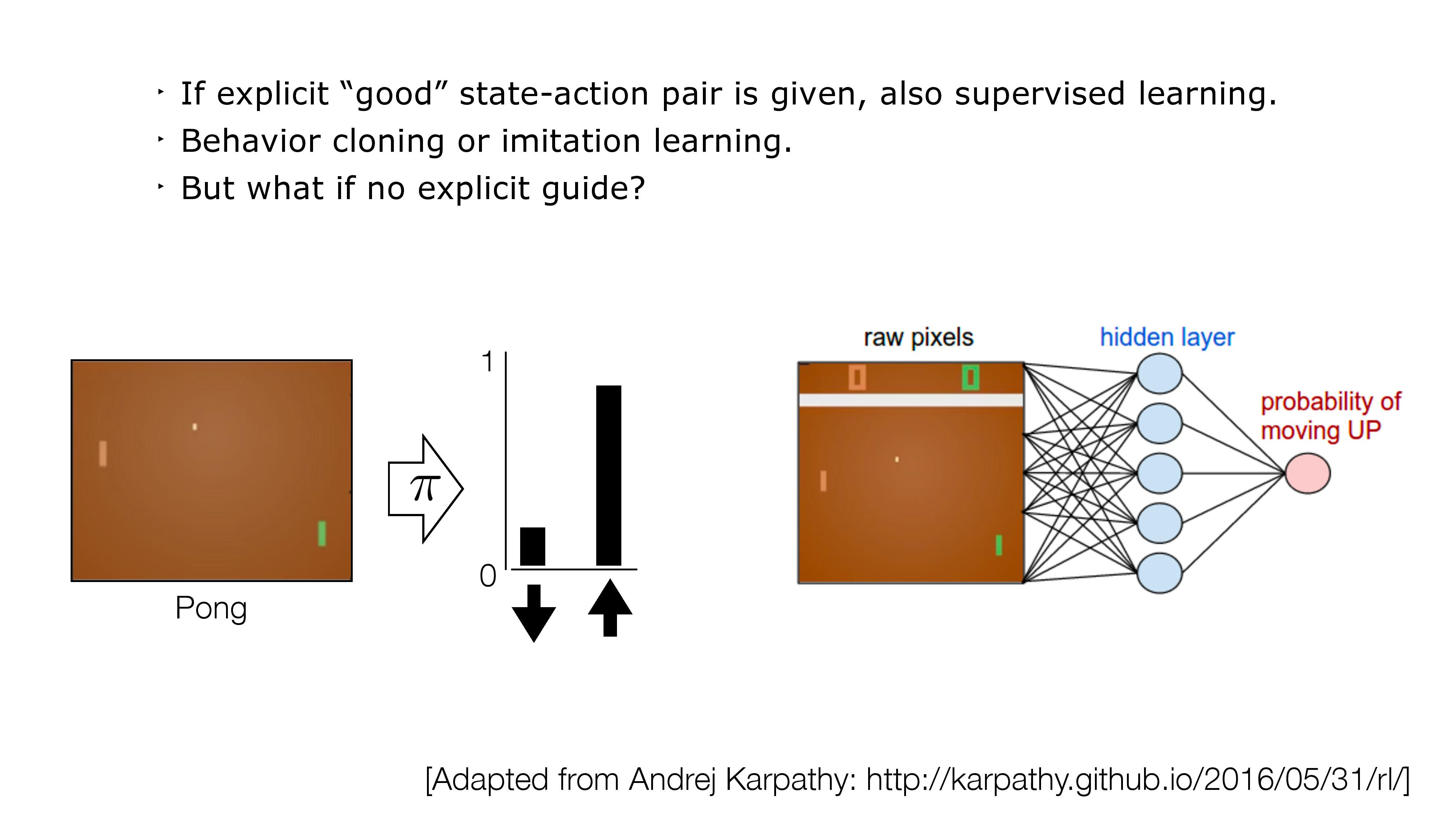
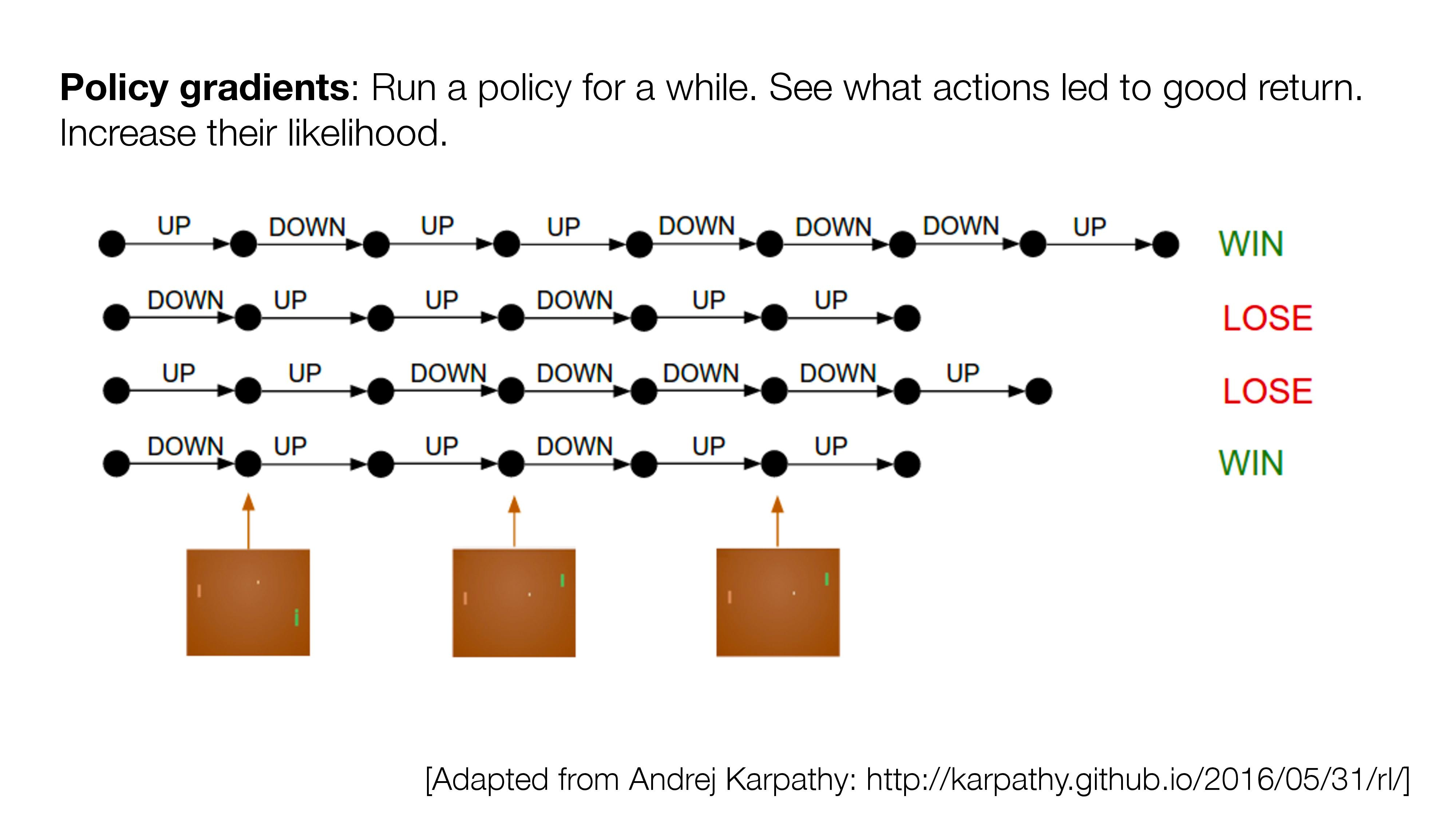
- If no direct supervision is available?
- Strictly RL setting. Interact, observe, get data, use rewards as "coy" supervision signal.
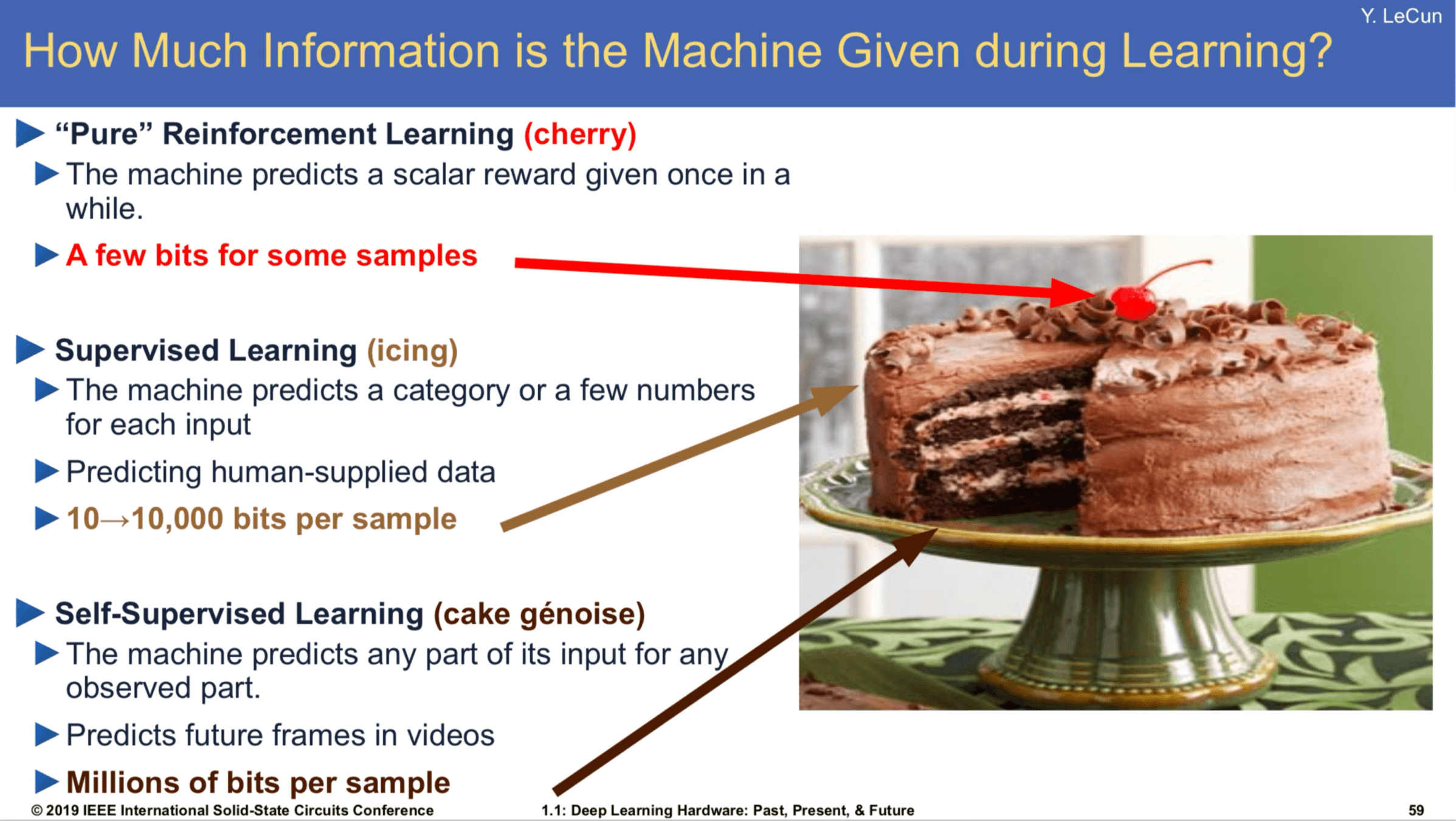
[Slide Credit: Yann LeCun]
Reinforcement learning has a lot of challenges:
- Data can be very expensive/tricky to get
- sim-to-real gap
- sparse rewards
- exploration-exploitation trade-off
- catastrophic forgetting
- Learning can be very inefficient
- temporal process, compound error
- super high variance
- learning process hard to stabilize
...
Summary
- We saw, last week, how to find good in a known MDP: these are policies with high cumulative expected reward.
- In reinforcement learning, we assume we are interacting with an unknown MDP, but we still want to find a good policy. We will do so via estimating the Q value function.
- One problem is how to select actions to gain good reward while learning. This “exploration vs exploitation” problem is important.
- Q-learning, for discrete-state problems, will converge to the optimal value function (with enough exploration).
- “Deep Q learning” can be applied to continuous-state or large discrete-state problems by using a parameterized function to represent the Q-values.
Thanks!
We'd love to hear your thoughts.
6.390 IntroML (Spring25) - Lecture 11 Reinforcement Learning
By Shen Shen


