

Lecture 6: Neural Networks II
Shen Shen
March 7, 2025
11am, Room 10-250
Intro to Machine Learning

Outline
- Recap: Multi-layer perceptrons, expressiveness
- Forward pass (to use/evaluate)
-
Backward pass (to learn parameters/weights)
- Back-propagation: (gradient descent & the chain rule)
- Practical gradient issues and remedies
Outline
- Recap: Multi-layer perceptrons, expressiveness
- Forward pass (to use/evaluate)
- Backward pass (to learn parameters/weights)
- Back-propagation: (gradient descent & the chain rule)
- Practical gradient issues and remedies
A neuron:
\(w\): what the algorithm learns
- \(x\): input (a single datapoint)
a = f(z)
\Sigma
- \(a\): post-activation output
- \(f\): activation function
- \(w\): weights (i.e. parameters)
- \(z\): pre-activation output
\(f\): what we engineers choose
\dots
x_1
x_2
x_d
x = \left[ \begin{array}{c}
\\
\\
\\
\\
\\
\\
\\
\end{array} \right]
w_1
w_d
\dots
w_2
= w^Tx
z
f(\cdot)
= f(w^Tx)
\(z\): scalar
\(a\): scalar
Choose activation \(f(z)=z\)
learnable parameters (weights)
e.g. linear regressor represented as a computation graph
= z
= w^Tx
w_1
w_d
\dots
x_1
x_2
x_d
\dots
x = \left[ \begin{array}{c}
\\
\\
\\
\\
\\
\\
\\
\end{array} \right]
w_2
\Sigma
f(\cdot)
g
z
neuron
Choose activation \(f(z)=\sigma(z)\)
learnable parameters (weights)
e.g. linear logistic classifier represented as a computation graph
= \sigma(z)
= w^Tx
w_1
w_d
\dots
x_1
x_2
x_d
\dots
w_2
\Sigma
f(\cdot)
g
z
x = \left[ \begin{array}{c}
\\
\\
\\
\\
\\
\\
\\
\end{array} \right]
neuron
\dots
A layer:
learnable weights
A layer:
a^1
z^1
\Sigma
f(\cdot)
z^2
\Sigma
f(\cdot)
a^2
z^m
a^m
\Sigma
f(\cdot)
\dots
x_1
x_2
x_d
- (# of neurons) = (layer's output dimension).
- typically, all neurons in one layer use the same activation \(f\) (if not, uglier algebra).
- typically fully connected, where all \(x_i\) are connected to all \(z^j,\) meaning each \(x_i\) influences every \(a^j\) eventually.
- typically, no "cross-wiring", meaning e.g. \(z^1\) won't affect \(a^2.\) (the output layer may be an exception if softmax is used.)
\dots
layer
linear combo
activations
A (fully-connected, feed-forward) neural network
\dots
\dots
layer
\dots
x_1
x_2
x_d
input
\Sigma
f(\cdot)
\Sigma
f(\cdot)
\Sigma
f(\cdot)
\Sigma
f(\cdot)
\Sigma
f(\cdot)
\Sigma
f(\cdot)
\Sigma
f(\cdot)
neuron
learnable weights
We choose:
- # of layers
- # of neurons in each layer
- activation \(f\) in each layer
hidden
output
(aka, multi-layer perceptrons MLP)
\sigma_1 = \sigma(5 x_1 -5 x_2 + 1)
\sigma_2 = \sigma(-5 x_1 + 5 x_2 + 1)
\(-3(\sigma_1 +\sigma_2)\)
recall this example
x_1
x_2
1
\Sigma
f(\cdot)
\Sigma
f(\cdot)
\Sigma
f(\cdot)
\(f =\sigma(\cdot)\)
\(f(\cdot) \) identity function
Recall
W^1
W^2
\sigma_1 = \sigma(5 x_1 -5 x_2 + 1)
\sigma_2 = \sigma(-5 x_1 + 5 x_2 + 1)
5
-5
1
-5
5
1
-3
-3
\(-3(\sigma_1 +\sigma_2)\)
Outline
- Recap: Multi-layer perceptrons, expressiveness
- Forward pass (to use/evaluate)
- Backward pass (to learn parameters/weights)
- Back-propagation: (gradient descent & the chain rule)
- Practical gradient issues and remedies
- Activation \(f\) is chosen as the identity function
- Evaluate the loss \(\mathcal{L} = (g^{(i)}-y^{(i)})^2\)
- Repeat for each data point, average the sum of \(n\) individual losses
e.g. forward-pass of a linear regressor
y^{(i)}
f(\cdot)
\underbrace{\quad \quad \quad }
\dots
= w^Tx
w_1
w_d
\dots
w_2
\Sigma
z
= z
g
\dots
x^{(i)}_1
x^{(i)}_2
x^{(i)}_d
x^{(i)} \quad = \left[ \begin{array}{c}
\\
\\
\\
\\
\\
\\
\\
\end{array} \right]
\mathcal{L}(g, y)
\mathcal{L}(g, y)
\mathcal{L}(g, y)
\dots
\dots
\dots
n
- Activation \(f\) is chosen as the sigmoid function
- Evaluate the loss \(\mathcal{L} = - [y^{(i)} \log g^{(i)}+\left(1-y^{(i)}\right) \log \left(1-g^{(i)}\right)]\)
- Repeat for each data point, average the sum of \(n\) individual losses
e.g. forward-pass of a linear logistic classifier
y^{(i)}
f(\cdot)
\underbrace{\quad \quad \quad }
\dots
= w^Tx
w_1
w_d
\dots
w_2
\Sigma
z
=\sigma(z)
g
\dots
x^{(i)}_1
x^{(i)}_2
x^{(i)}_d
x^{(i)} \quad = \left[ \begin{array}{c}
\\
\\
\\
\\
\\
\\
\\
\end{array} \right]
\mathcal{L}(g, y)
\mathcal{L}(g, y)
\mathcal{L}(g, y)
\dots
\dots
\dots
n
x^{(1)}
y^{(1)}
f^1
\begin{aligned}
& W^1 \\
\end{aligned}
\begin{aligned}
& W^2 \\
\end{aligned}
\begin{aligned}
& W^L \\
\end{aligned}
f^2
f^L
g^{(1)}
\(\dots\)
f^2\left(\hspace{2cm}; \mathbf{W}^2\right)
f^1(\mathbf{x}^{(i)}; \mathbf{W}^1)
f^L\left(\dots \hspace{3.5cm}; \dots \mathbf{W}^L\right)
Forward pass: evaluate, given the current parameters
- the model outputs \(g^{(i)}\) =
- the loss incurred on the current data \(\mathcal{L}(g^{(i)}, y^{(i)})\)
- the training error \(J = \frac{1}{n} \sum_{i=1}^{n}\mathcal{L}(g^{(i)}, y^{(i)})\)
\mathcal{L}(g^{(1)}, y^{(1)})
\mathcal{L}(g, y)
\mathcal{L}(g^{(n)}, y^{(n)})
\underbrace{\quad \quad \quad \quad \quad }
\dots
\dots
\dots
n
linear combination
loss function
(nonlinear) activation
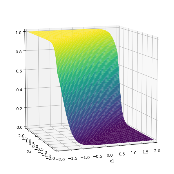
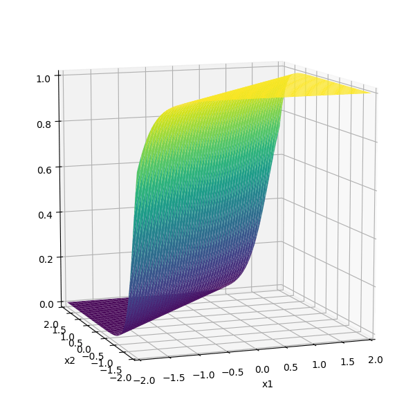
compositions of ReLU(s) can be quite expressive
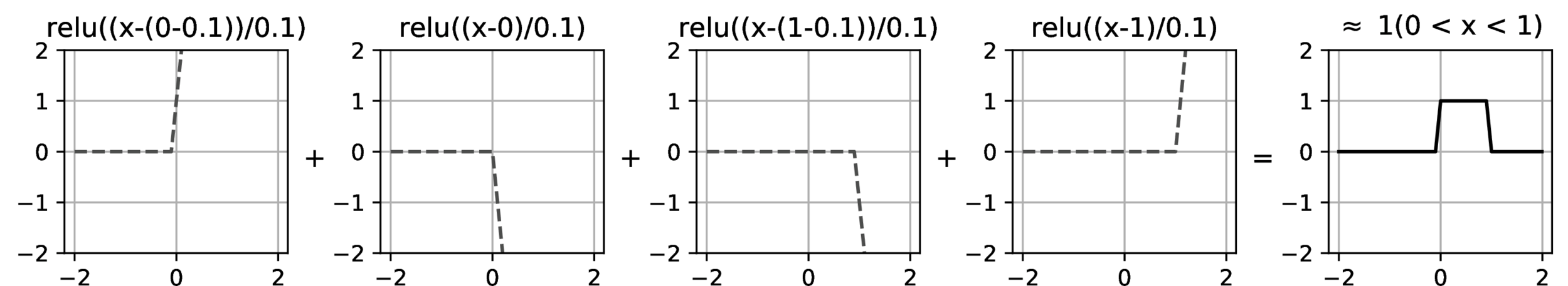
in fact, asymptotically, can approximate any function!
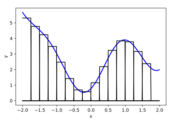
image credit: Phillip Isola
Recall:
Outline
- Recap: Multi-layer perceptrons, expressiveness
- Forward pass (to use/evaluate)
-
Backward pass (to learn parameters/weights)
- Back-propagation: (gradient descent & the chain rule)
- Practical gradient issues and remedies
\mathcal{L}(g, y)
\mathcal{L}(g, y)
\underbrace{\quad \quad \quad } \\ n
\mathcal{L}(g, y)
\dots
x_1
x_2
x_d
x^{(i)} \quad = \left[ \begin{array}{c}
\\
\\
\\
\\
\\
\\
\\
\end{array} \right]
stochastic gradient descent to learn a linear regressor
\dots
y^{(i)}
\dots
\dots
- Randomly pick a data point \((x^{(i)}, y^{(i)})\)
- Evaluate the gradient \(\nabla_{w} \mathcal{L(g^{(i)},y^{(i)})}\)
- Update the weights \(w \leftarrow w - \eta \nabla_w \mathcal{L(g^{(i)},y^{(i)}})\)

w
\left[ \begin{array}{c}
\\
\\
\\
\\
\\
\\
\\
\end{array} \right]
= w^Tx
\Sigma
w_1
w_2
\dots
w_d
w_1
w_2
\dots
w_d
=
\nabla_{w} \mathcal{L(g^{(i)},y^{(i)})}
g
\mathcal{L}(g, y)
\dots
x_1
x_2
x_d
x \quad = \left[ \begin{array}{c}
\\
\\
\\
\\
\\
\\
\\
\end{array} \right]
for simplicity, say the dataset has only one data point \((x,y)\)
y
\left[ \begin{array}{c}
\\
\\
\\
\\
\\
\\
\\
\end{array} \right]
\Sigma
w_1
w_2
\dots
w_d
y \in \mathbb{R}
x \in \mathbb{R^d}
w \in \mathbb{R^d}
= \frac{\partial \mathcal{L}(g,y)}{\partial w}
\nabla_{w} \mathcal{L(g,y)}
= x \cdot 2(g - y)
\frac{\partial g}{\partial w}
= \frac{\partial[(g - y)^2] }{\partial w}
= \frac{\partial[(w^T x - y)^2] }{\partial w}
\nabla_{w} \mathcal{L(g,y)}
\frac{\partial \mathcal{L}}{\partial g}
w
=
\nabla_{w} \mathcal{L(g,y)}
= w^Tx
g
example on black-board
- default choice in hidden layers
- very simple function form, so is the gradient.
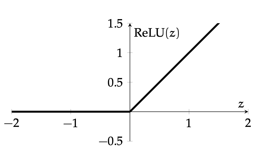
Recall:
\frac{\partial \text{ReLU}(z)}{\partial z}=\left\{\begin{array}{lll}
0, & \text {if } z<0 \\
1, & \text{otherwise}
\end{array}\right.
\text{ReLU}
\dots
x_1
x_2
x_d
x \quad = \left[ \begin{array}{c}
\\
\\
\\
\\
\\
\\
\\
\end{array} \right]
now, slightly more interesting activation:
y
\left[ \begin{array}{c}
\\
\\
\\
\\
\\
\\
\\
\end{array} \right]
= w^Tx
\Sigma
z
w_1
w_2
\dots
w_d
= \frac{\partial \mathcal{L}(g,y)}{\partial w}
\nabla_{w} \mathcal{L(g,y)}
= x \cdot \frac{\partial[(\text{ReLU}(z))] }{\partial z} \cdot 2(g - y)
\frac{\partial g}{\partial z}
\frac{\partial z}{\partial w}
= \frac{\partial[(g - y)^2] }{\partial w}
\nabla_{w} \mathcal{L(g,y)}
\frac{\partial \mathcal{L}}{\partial g}
w
=
\nabla_{w} \mathcal{L(g,y)}
g
= \text{ReLU}(z)
example on black-board
\mathcal{L}(g, y)
y \in \mathbb{R}
x \in \mathbb{R^d}
w \in \mathbb{R^d}
- Randomly pick a data point \((x^{(i)}, y^{(i)})\)
- Evaluate the gradient \(\nabla_{W^2} \mathcal{L(g^{(i)},y^{(i)})}\)
- Update the weights \(W^2 \leftarrow W^2 - \eta \nabla_{W^2} \mathcal{L(g^{(i)},y^{(i)}})\)
x^{(i)}
y^{(i)}
f^1
\begin{aligned}
& W^1 \\
\end{aligned}
\begin{aligned}
& W^2 \\
\end{aligned}
\begin{aligned}
& W^L \\
\end{aligned}
f^2
f^L
g^{(i)}
\(\dots\)
\mathcal{L}(g^{(i)}, y^{(i)})
\mathcal{L}(g, y)
\mathcal{L}(g^{(n)}, y^{(n)})
\underbrace{\quad \quad \quad \quad \quad }
\dots
\dots
\dots
\(\nabla_{W^2} \mathcal{L(g^{(i)},y^{(i)})}\)
n
Backward pass: run SGD to update all parameters
- e.g. to update \(W^2\)
x
\(\dots\)
y
f^1
\begin{aligned}
& W^1 \\
\end{aligned}
\begin{aligned}
& W^2 \\
\end{aligned}
\begin{aligned}
& W^L \\
\end{aligned}
f^2
f^L
\mathcal{L}(g,y)
g
\(\nabla_{W^2} \mathcal{L(g,y)}\)
Backward pass: run SGD to update all parameters
- e.g. to update \(W^2\)
Evaluate the gradient \(\nabla_{W^2} \mathcal{L(g,y)}\)
Update the weights \(W^2 \leftarrow W^2 - \eta \nabla_{W^2} \mathcal{L(g,y})\)
x
\(\dots\)
y
f^1
\begin{aligned}
& W^1 \\
\end{aligned}
\begin{aligned}
& W^2 \\
\end{aligned}
\begin{aligned}
& W^L \\
\end{aligned}
f^2
f^L
\mathcal{L}(g,y)
g
\underbrace{\hspace{4.7cm}}
Z^L
A^2
Z^2
A^1
Z^1
\frac{\partial \mathcal{L}(g,y)}{\partial W^2}
\frac{\partial \mathcal{L}(g,y)}{\partial g}
\frac{\partial g}{\partial Z^{L}}
\frac{\partial Z^3}{\partial A^{2}}\frac{\partial A^4}{\partial Z^{3}} \dots \frac{\partial Z^L}{\partial A^{L-1}}
\frac{\partial A^2}{\partial Z^{2}}
\frac{\partial Z^2}{\partial W^{2}}
\frac{\partial \mathcal{L}(g,y)}{\partial Z^2}
\underbrace{\hspace{4cm}}
\frac{\partial \mathcal{L}(g,y)}{\partial W^2}
how to find
?
x
y
f^1
\begin{aligned}
& W^1 \\
\end{aligned}
\begin{aligned}
& W^2 \\
\end{aligned}
\mathcal{L}(g,y)
g
\(\nabla_{W^1} \mathcal{L(g,y)}\)
Now, how to update \(W^1?\)
\(\dots\)
\begin{aligned}
& W^L \\
\end{aligned}
f^2
f^L
Evaluate the gradient \(\nabla_{W^1} \mathcal{L(g,y)}\)
Update the weights \(W^1 \leftarrow W^1 - \eta \nabla_{W^1} \mathcal{L(g,y})\)
\frac{\partial \mathcal{L}(g,y)}{\partial W^1}
x
\(\dots\)
y
f^1
\begin{aligned}
& W^1 \\
\end{aligned}
\begin{aligned}
& W^2 \\
\end{aligned}
\begin{aligned}
& W^L \\
\end{aligned}
f^2
f^L
\mathcal{L}(g,y)
g
Z^L
A^2
Z^2
A^1
Z^1
\frac{\partial \mathcal{L}(g,y)}{\partial g}
\frac{\partial g}{\partial Z^{L}}
\frac{\partial Z^3}{\partial A^{2}}\frac{\partial A^4}{\partial Z^{3}} \dots \frac{\partial Z^L}{\partial A^{L-1}}
\frac{\partial A^2}{\partial Z^{2}}
\frac{\partial \mathcal{L}(g,y)}{\partial Z^2}
\underbrace{\hspace{4cm}}
\frac{\partial Z^2}{\partial W^{2}}
\underbrace{\hspace{4.7cm}}
\frac{\partial \mathcal{L}(g,y)}{\partial W^2}
how to find
?
Previously, we found
\underbrace{\hspace{6.5cm}}
\frac{\partial Z^2}{\partial A^{1}}
\frac{\partial A^1}{\partial Z^{1}}
\frac{\partial Z^1}{\partial W^{1}}
x
\(\dots\)
y
f^1
\begin{aligned}
& W^1 \\
\end{aligned}
\begin{aligned}
& W^2 \\
\end{aligned}
\begin{aligned}
& W^L \\
\end{aligned}
f^2
f^L
\mathcal{L}(g,y)
g
Z^L
A^2
Z^2
A^1
Z^1
\frac{\partial \mathcal{L}(g,y)}{\partial g}
\frac{\partial g}{\partial Z^{L}}
\frac{\partial Z^3}{\partial A^{2}}\frac{\partial A^4}{\partial Z^{3}} \dots \frac{\partial Z^L}{\partial A^{L-1}}
\frac{\partial A^2}{\partial Z^{2}}
\frac{\partial \mathcal{L}(g,y)}{\partial Z^2}
\underbrace{\hspace{4cm}}
\frac{\partial \mathcal{L}(g,y)}{\partial W^1}
how to find
Now
\frac{\partial \mathcal{L}(g,y)}{\partial W^1}
x
\(\dots\)
y
f^1
\begin{aligned}
& W^1 \\
\end{aligned}
\begin{aligned}
& W^2 \\
\end{aligned}
\begin{aligned}
& W^L \\
\end{aligned}
f^2
f^L
\mathcal{L}(g,y)
g
Z^L
A^2
Z^2
A^1
Z^1
\frac{\partial \mathcal{L}(g,y)}{\partial g}
\frac{\partial g}{\partial Z^{L}}
\frac{\partial Z^3}{\partial A^{2}}\frac{\partial A^4}{\partial Z^{3}} \dots \frac{\partial Z^L}{\partial A^{L-1}}
\frac{\partial A^2}{\partial Z^{2}}
\frac{\partial \mathcal{L}(g,y)}{\partial Z^2}
\underbrace{\hspace{4cm}}
\underbrace{\hspace{4.7cm}}
\frac{\partial Z^2}{\partial W^{2}}
\frac{\partial \mathcal{L}(g,y)}{\partial W^2}
back propagation: reuse of computation
\underbrace{\hspace{6.5cm}}
\frac{\partial Z^2}{\partial A^{1}}
\frac{\partial A^1}{\partial Z^{1}}
\frac{\partial Z^1}{\partial W^{1}}
x
\(\dots\)
y
f^1
\begin{aligned}
& W^1 \\
\end{aligned}
\begin{aligned}
& W^2 \\
\end{aligned}
\begin{aligned}
& W^L \\
\end{aligned}
f^2
f^L
\mathcal{L}(g,y)
g
Z^L
A^2
Z^2
A^1
Z^1
\frac{\partial \mathcal{L}(g,y)}{\partial g}
\frac{\partial g}{\partial Z^{L}}
\frac{\partial Z^3}{\partial A^{2}}\frac{\partial A^4}{\partial Z^{3}} \dots \frac{\partial Z^L}{\partial A^{L-1}}
\frac{\partial A^2}{\partial Z^{2}}
\frac{\partial \mathcal{L}(g,y)}{\partial Z^2}
\underbrace{\hspace{4cm}}
\frac{\partial \mathcal{L}(g,y)}{\partial W^1}
\underbrace{\hspace{4.7cm}}
\frac{\partial Z^2}{\partial W^{2}}
\frac{\partial \mathcal{L}(g,y)}{\partial W^2}
back propagation: reuse of computation
Outline
- Recap: Multi-layer perceptrons, expressiveness
- Forward pass (to use/evaluate)
-
Backward pass (to learn parameters/weights)
- Back-propagation: (gradient descent & the chain rule)
- Practical gradient issues and remedies
\text{ReLU}
\dots
x_1
x_2
x_d
x \quad = \left[ \begin{array}{c}
\\
\\
\\
\\
\\
\\
\\
\end{array} \right]
Let's revisit this:
y
\left[ \begin{array}{c}
\\
\\
\\
\\
\\
\\
\\
\end{array} \right]
= w^Tx
\Sigma
z
w_1
w_2
\dots
w_d
= \frac{\partial \mathcal{L}(g,y)}{\partial w}
\nabla_{w} \mathcal{L(g,y)}
= x \cdot \frac{\partial[(\text{ReLU}(z))] }{\partial z} \cdot 2(g - y)
\frac{\partial g}{\partial z}
\frac{\partial z}{\partial w}
= \frac{\partial[(g - y)^2] }{\partial w}
\nabla_{w} \mathcal{L(g,y)}
\frac{\partial \mathcal{L}}{\partial g}
w
=
\nabla_{w} \mathcal{L(g,y)}
g
= \text{ReLU}(z)
example on black-board
\mathcal{L}(g, y)
y \in \mathbb{R}
x \in \mathbb{R^d}
w \in \mathbb{R^d}
\mathcal{L}(g, y)
\dots
x_1
x_2
x_d
x = \left[ \begin{array}{c}
\\
\\
\\
\\
\\
\\
\\
\end{array} \right]
y
\Sigma
\Sigma
\text{ReLU}
\text{ReLU}
\begin{bmatrix}
a_{1}^1 \\[3ex]
a_2^1
\end{bmatrix}
\Sigma
g
\text{ReLU}
W^1
W^2
z^{2}
z_{1}^{1}
z_{2}^{1}
now, slightly more complex network:
example on black-board
\mathcal{L}(g, y)
\dots
x_1
x_2
x_d
x = \left[ \begin{array}{c}
\\
\\
\\
\\
\\
\\
\\
\end{array} \right]
y
\Sigma
\Sigma
\text{ReLU}
\text{ReLU}
\begin{bmatrix}
a_{1}^1 \\[3ex]
a_2^1
\end{bmatrix}
\Sigma
g
\text{ReLU}
W^1
W^2
z^{2}
z_{1}^{1}
z_{2}^{1}
now, slightly more complex network:
example on black-board
if \(z^2 > 0\) and \(z_1^1 < 0\), some weights (grayed-out ones) won't get updated
\mathcal{L}(g, y)
\dots
x_1
x_2
x_d
x = \left[ \begin{array}{c}
\\
\\
\\
\\
\\
\\
\\
\end{array} \right]
y
\Sigma
\Sigma
\text{ReLU}
\text{ReLU}
\begin{bmatrix}
a_{1}^1 \\[3ex]
a_2^1
\end{bmatrix}
\Sigma
g
\text{ReLU}
W^1
W^2
z^{2}
z_{1}^{1}
z_{2}^{1}
now, slightly more complex network:
example on black-board
if \(z^2 < 0\), no weights get updated

- Width: # of neurons in layers
- Depth: # of layers
- Typically, increasing either the width or depth (with non-linear activation) makes the model more expressive, but it also increases the risk of overfitting.
However, in the realm of neural networks, the precise nature of this relationship remains an active area of research—for example, phenomena like the double-descent curve and scaling laws
- To combat vanishing gradient is another reason networks are typically wide.
- Still have vanishing gradient tendency if the network is deep.
Recall:
\mathcal{L}(g, y)
\dots
x_1
x_2
x_d
x = \left[ \begin{array}{c}
\\
\\
\\
\\
\\
\\
\\
\end{array} \right]
y
\Sigma
\Sigma
\text{ReLU}
\text{ReLU}
\begin{bmatrix}
a_{1}^1 \\[3ex]
a_2^1
\end{bmatrix}
\Sigma
g
\text{ReLU}
W^1
W^2
z^{2}
z_{1}^{1}
z_{2}^{1}
Residual (skip) connection :
example on black-board
Now, \(g= a^1 + \text{ReLU}(z^2),\)
even if \(z^2 < 0\), with skip connection, weights in earlier layers can still get updated
a^1
\underbrace{}
Summary
- We saw that multi-layer perceptrons are a way to automatically find good features/transformations for us!
- In fact, roughly speaking, can asymptotically learn anything (universal approximation theorem).
- How to learn? Still just (stochastic) gradient descent!
- Thanks to the layered structure, turns out we can reuse lots of computation in gradient descent update -- back propagation.
- Practically, there can be numerical gradient issues. There're remedies, e.g. via having lots of neurons, or, via residual connections.
Thanks!
We'd love to hear your thoughts.
6.390 IntroML (Spring25) - Lecture 6 Neural Networks II
By Shen Shen


