
Lecture 11: Reinforcement Learning
Intro to Machine Learning


- \(\mathcal{S}\) : state space, contains all possible states \(s\).
- \(\mathcal{A}\) : action space, contains all possible actions \(a\).
- \(\mathrm{T}\left(s, a, s^{\prime}\right)\) : the probability of transition from state \(s\) to \(s^{\prime}\) when action \(a\) is taken.
- \(\mathrm{R}(s, a)\) : reward, takes in a (state, action) pair and returns a reward.
- \(\gamma \in [0,1]\): discount factor, a scalar.
- \(\pi{(s)}\) : policy, takes in a state and returns an action.
The goal of an MDP is to find a "good" policy.
MDP: Definition and terminologies
In 6.390,
- \(\mathcal{S}\) and \(\mathcal{A}\) are small discrete sets, unless otherwise specified.
- \(s^{\prime}\) and \(a^{\prime}\) are short-hand for the next-timestep state and action.
- \(\mathrm{R}(s, a)\) is deterministic and bounded.
- \(\pi(s)\) is deterministic.
Recall
finite-horizon Bellman recursions
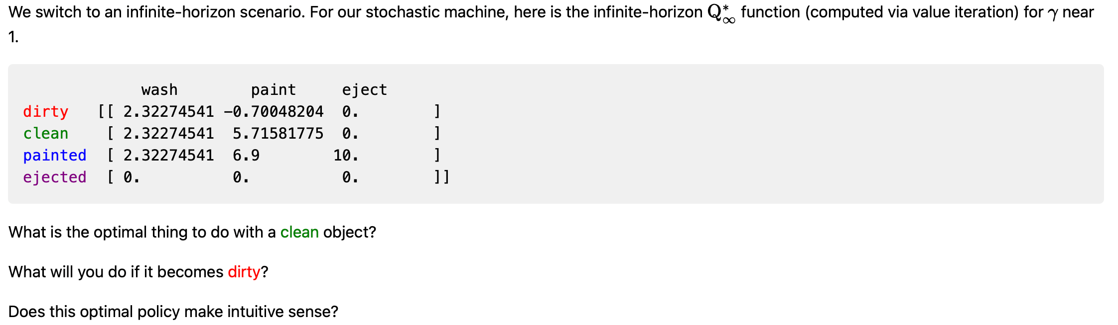
infinite-horizon Bellman equations
\mathrm{V}^\pi_{\infty}(s)= \mathrm{R}(s, \pi(s))+ \gamma \sum_{s^{\prime}} \mathrm{T}\left(s, \pi(s), s^{\prime}\right) \mathrm{V}^\pi_{\infty}\left(s^{\prime}\right)
\mathrm{V}_{h}^\pi(s)= \mathrm{R}(s, \pi(s))+ \gamma \sum_{s^{\prime}} \mathrm{T}\left(s, \pi(s), s^{\prime}\right) \mathrm{V}_{h-1}^\pi\left(s^{\prime}\right)
\pi(s)
\mathrm{V}^{\pi}_{h}(s)
Policy Evaluation
Use the definition and sum up expected rewards:
Or, leverage the recursive structure:
\mathrm{V}_h^\pi(s):=\mathbb{E}\left[\sum_{t=0}^{h-1} \gamma^t \mathrm{R}\left(s_t, \pi\left(s_t\right)\right) \mid s_0=s, \pi\right]
1️⃣
2️⃣
3️⃣
Recall
the immediate reward for taking the policy-prescribed action \(\pi(s)\) in state \(s\).
horizon-\(h\) value in state \(s\): the expected sum of discounted rewards, starting in state \(s\) and following policy \(\pi\) for \(h\) steps.
\((h-1)\) horizon future value at a next state \(s^{\prime}\)
sum of future values weighted by the probability of reaching that next state \(s^{\prime}\)
discounted by \(\gamma\)
2️⃣
Recall
\mathrm{V}_{h}^\pi(s)= \mathrm{R}(s, \pi(s))+ \gamma \sum_{s^{\prime}} \mathrm{T}\left(s, \pi(s), s^{\prime}\right) \mathrm{V}_{h-1}^\pi\left(s^{\prime}\right)
the optimal state-action value function \(\mathrm{Q}^*_h(s, a):\)
the expected sum of discounted rewards, obtained by
- starting in state \(s\)
- taking action \(a\), for one step
- acting optimally thereafter for the remaining \((h-1)\) steps
\(\mathrm{V}_h^*(s) = \max_{a} \big[\mathrm{R}(s, a) + \gamma \sum_{s'} \mathrm{T}(s, a, s') \mathrm{V}_{h-1}^*(s') \big]\)
\(=\max_{a}\left[\mathrm{Q}^*_{h}(s, a)\right]\)
\(\mathrm{Q}^*\) satisfies the Bellman recursion:
\(\mathrm{Q}^*_h (s, a)=\mathrm{R}(s, a)+\gamma \sum_{s^{\prime}} \mathrm{T}\left(s, a, s^{\prime} \right) \max _{a^{\prime}} \mathrm{Q}^*_{h-1}\left(s^{\prime}, a^{\prime}\right)\)
4️⃣
5️⃣
Recall
- for \(s \in \mathcal{S}, a \in \mathcal{A}\) :
- \(\mathrm{Q}_{\text {old }}(\mathrm{s}, \mathrm{a})=0\)
- while True:
- for \(s \in \mathcal{S}, a \in \mathcal{A}\) :
- \(\mathrm{Q}_{\text {new }}(s, a) \leftarrow \mathrm{R}(s, a)+\gamma \sum_{s^{\prime}} \mathrm{T}\left(s, a, s^{\prime}\right) \max _{a^{\prime}} \mathrm{Q}_{\text {old }}\left(s^{\prime}, a^{\prime}\right)\)
- if \(\max _{s, a}\left|Q_{\text {old }}(s, a)-Q_{\text {new }}(s, a)\right|<\epsilon:\)
- return \(\mathrm{Q}_{\text {new }}\)
- \(\mathrm{Q}_{\text {old }} \leftarrow \mathrm{Q}_{\text {new }}\)
Value Iteration
if we run this block \(h\) times and break, then the returns are \(\mathrm{Q}^*_h\)
\{
returns are \(\mathrm{Q}^*_{\infty}\)
Value iteration: iteratively invoke
\{
Recall
\(\mathrm{Q}^*_h (s, a)=\mathrm{R}(s, a)+\gamma \sum_{s^{\prime}} \mathrm{T}\left(s, a, s^{\prime} \right) \max _{a^{\prime}} \mathrm{Q}^*_{h-1}\left(s^{\prime}, a^{\prime}\right)\)
5️⃣
Outline
- Reinforcement learning setup
- Tabular Q-learning
- exploration vs. exploitation
- \(\epsilon\)-greedy action selection
- Fitted Q-learning
- (Policy gradient)
- Reinforcement learning setup
- Tabular Q-learning
- exploration vs. exploitation
- \(\epsilon\)-greedy action selection
- Fitted Q-learning
- (Policy gradient)
- transition probabilities are known
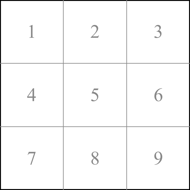
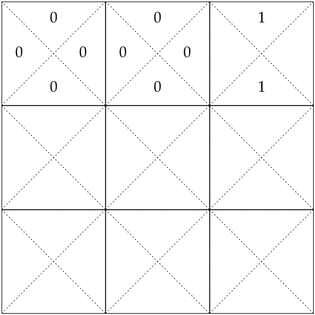
Mario in a grid-world v1.0
(Markov-decision-process version)

- 9 possible states
- 4 possible actions: {Up ↑, Down ↓, Left ←, Right →}
- rewards known
- discount factor \(\gamma = 0.9\)
80\%
20\%

e.g., \(\mathrm{T}\left(7, \uparrow, 4\right) = 1\)
\(\mathrm{T}\left(9, \rightarrow, 9\right) = 1\)
\(\mathrm{T}\left(6, \uparrow, 3\right) = 0.8\)
\(\mathrm{T}\left(6, \uparrow, 2\right) = 0.2\)
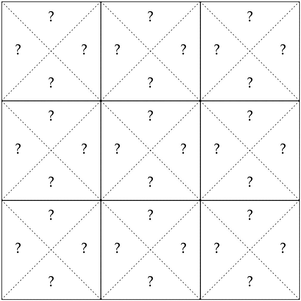
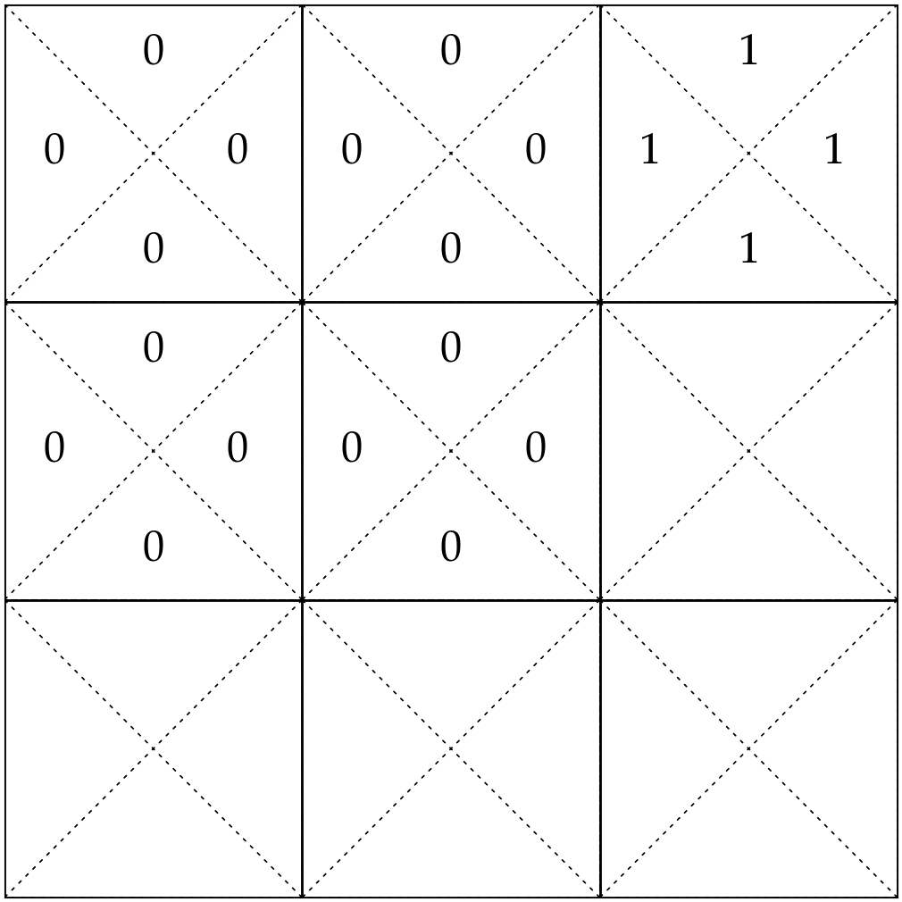
- transition probabilities are unknown
Mario in a grid-world v2.0
(reinforcement learning version)
- 9 possible states
- 4 possible actions: {Up ↑, Down ↓, Left ←, Right →}
- rewards unknown
- discount factor \(\gamma = 0.9\)
?
?
?
\dots
?
e.g., \(\mathrm{T}\left(7, \uparrow, 4\right) = ?\)
\(\mathrm{T}\left(9, \rightarrow, 9\right) = ?\)
\(\mathrm{T}\left(6, \uparrow, 3\right) = ?\)
\(\mathrm{T}\left(6, \uparrow, 2\right) = ?\)
- \(\mathcal{S}\) : state space, contains all possible states \(s\).
- \(\mathcal{A}\) : action space, contains all possible actions \(a\).
- \(\mathrm{T}\left(s, a, s^{\prime}\right)\) : the probability of transition from state \(s\) to \(s^{\prime}\) when action \(a\) is taken.
- \(\mathrm{R}(s, a)\) : reward, takes in a (state, action) pair and returns a reward.
- \(\gamma \in [0,1]\): discount factor, a scalar.
- \(\pi{(s)}\) : policy, takes in a state and returns an action.
The goal of an MDP problem is to find a "good" policy.
Markov Decision Processes - Definition and terminologies
Reinforcement Learning
RL
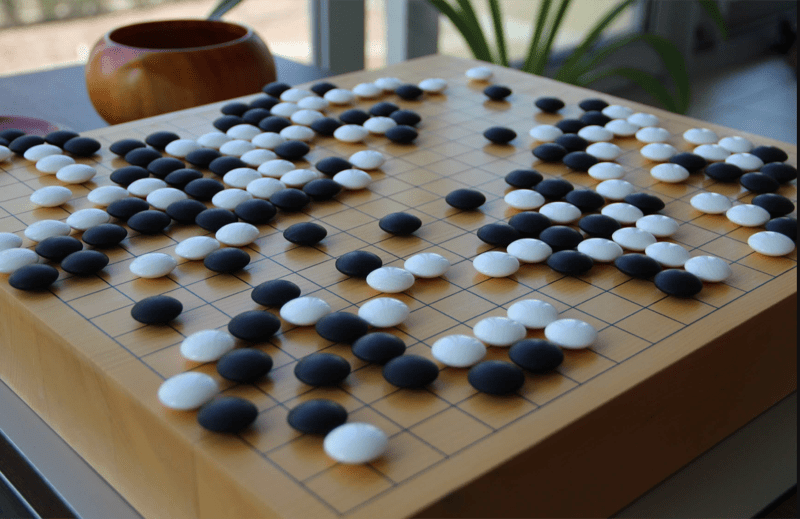
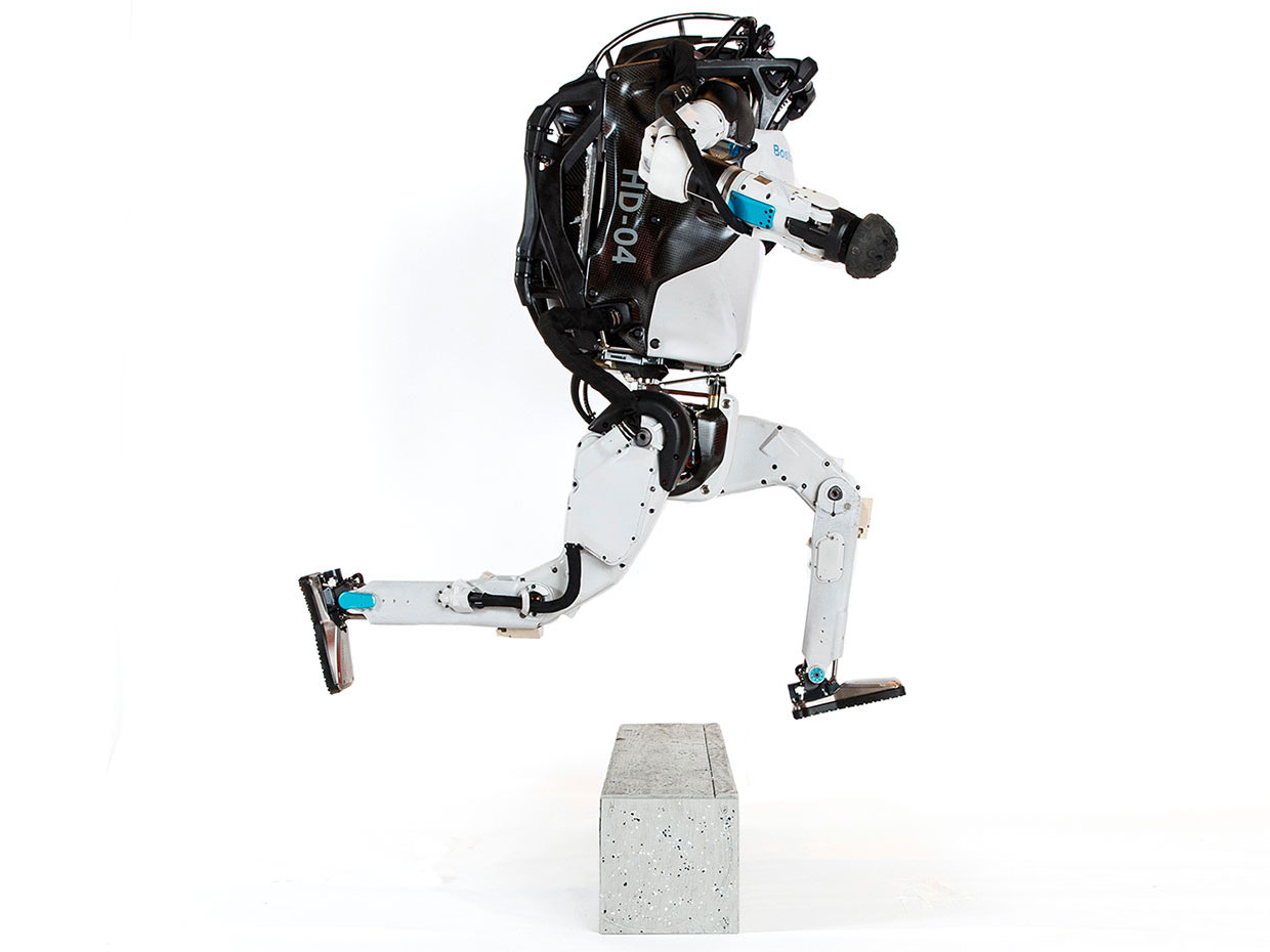
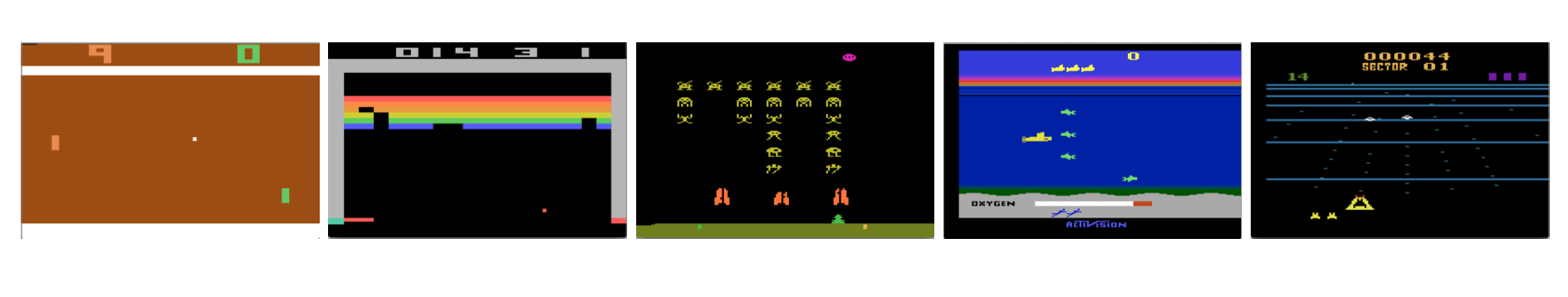
Reinforcement learning is very general:
robotics
games
social sciences
chatbots (RLHF)
health care

...
Model-based RL: Learn the MDP tuple
1. Collect experiences \((s, a, r, s^{\prime})\)
2. Estimate \(\mathrm{\hat{T}}\), \(\mathrm{\hat{R}}\)
3. Solve \(\langle\mathcal{S}, \mathcal{A}, \mathrm{\hat{T}}, \mathrm{\hat{R}}, \gamma\rangle\) via e.g. Value Iteration
\(\frac{\text{observed} (6, \uparrow, 2) } {\text{total} (6,\uparrow)\text{ play count}}\)
e.g. \({\mathrm{\hat{T}}}(6,\uparrow, 2 ) \approx \)
observed reward received from (6, \(\uparrow\))
e.g. \({\mathrm{\hat{R}}}(6,\uparrow ) =\)
\(\gamma = 0.9\)
Unknown transition:
?
?
?
\dots
?
Unknown rewards
\(\dots\)
\((1,\uparrow)\)
0
1
\((3,\uparrow)\)
1
3
\((3,\downarrow)\)
1
6
\(\dots\)
\((6,\uparrow)\)
-10
3
\(\dots\)
\((6,\uparrow)\)
-10
2

\((s, a)\)
\(r \)
\(s^{\prime}\)
\((1,\downarrow)\)
\(0\)
\(4\)

compounding error: if the learned MDP model is slightly wrong, our policy is doomed
do not explicitly learn MDP tuple
learn values (or policies) directly
- In RL we don't say hypothesis; we say model, value, or policy
Model in MDP/RL typically means the MDP tuple \(\langle\mathcal{S}, \mathcal{A}, \mathrm{T}, \mathrm{R}, \gamma\rangle\)
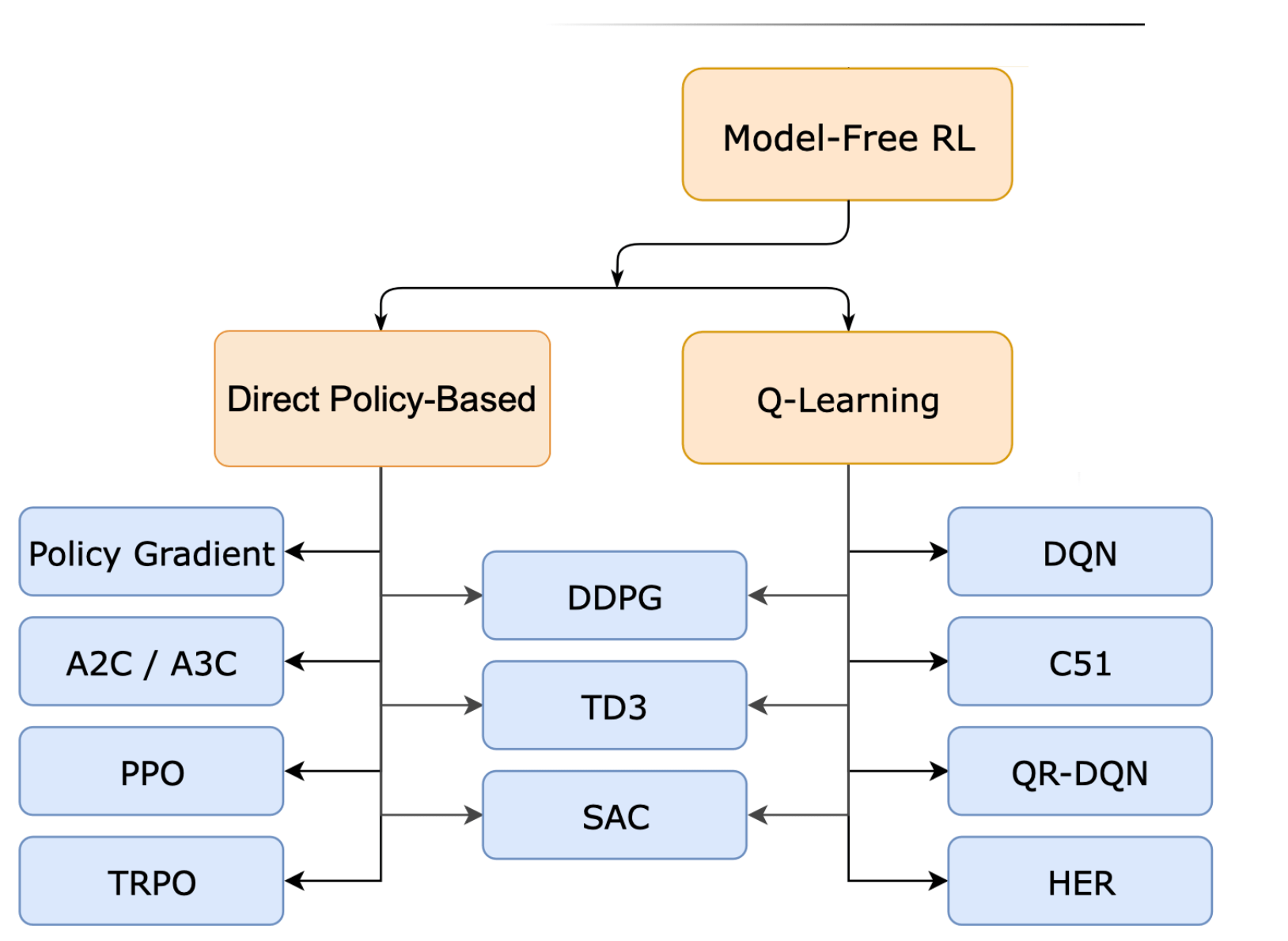
[A non-exhaustive, but useful taxonomy of algorithms in modern RL. Source]
We'll focus on (tabular) Q-learning
and to a lesser extent, touch on fitted Q-learning methods such as DQN
Direct Policy-Based
Outline
- Reinforcement learning setup
-
Tabular Q-learning
- exploration vs. exploitation
- \(\epsilon\)-greedy action selection
- Fitted Q-learning
- (Policy gradient)
Is it possible to get an optimal policy without learning transition or rewards explicitly?
Yes! We know one way already:
(Recall, from the MDP lab)
\pi_h^*(s)=\arg \max _a \mathrm{Q}^*_h(s, a)
Optimal policy \(\pi^*\) easily extracted from \(\mathrm{Q}^*\):
6️⃣
and doesn't value iteration rely on transition and rewards explicitly?
\(\mathrm{Q}_{\text {new }}(s, a) \leftarrow \mathrm{R}(s, a)+\gamma \sum_{s^{\prime}} \mathrm{T}\left(s, a, s^{\prime}\right) \max _{a^{\prime}} \mathrm{Q}_{\text {old }}\left(s^{\prime}, a^{\prime}\right)\)
Value Iteration
- for \(s \in \mathcal{S}, a \in \mathcal{A}\) :
- \(\mathrm{Q}_{\text {old }}(\mathrm{s}, \mathrm{a})=0\)
- while True:
- for \(s \in \mathcal{S}, a \in \mathcal{A}\) :
- \(\mathrm{Q}_{\text {new }}(s, a) \leftarrow \mathrm{R}(s, a)+\gamma \sum_{s^{\prime}} \mathrm{T}\left(s, a, s^{\prime}\right) \max _{a^{\prime}} \mathrm{Q}_{\text {old }}\left(s^{\prime}, a^{\prime}\right)\)
- if \(\max _{s, a}\left|Q_{\text {old }}(s, a)-Q_{\text {new }}(s, a)\right|<\epsilon:\)
- return \(\mathrm{Q}_{\text {new }}\)
- \(\mathrm{Q}_{\text {old }} \leftarrow \mathrm{Q}_{\text {new }}\)
But... didn't we arrive at \(\mathrm{Q}^*\) by value iteration,
- Indeed, value iteration relies on having full access to \(\mathrm{R}\) and \(\mathrm{T}\)
- Without \(\mathrm{R}\) and \(\mathrm{T}\), how about: execute \((s,a)\), observe \(r\) and \(s'\), and update:
(we'll see why this fails)
\(\mathrm{Q}_{\text {new }}(s, a) \leftarrow \mathrm{R}(s, a)+\gamma \sum_{s^{\prime}} \mathrm{T}\left(s, a, s^{\prime}\right) \max _{a^{\prime}} \mathrm{Q}_{\text {old }}\left(s^{\prime}, a^{\prime}\right)\)
immediate reward
future value, starting in state \(s'\) and acting optimally for \((h-1)\) steps
expected future value, weighted by the chance of landing in that particular future state \(s'\)
target
\(\mathrm{Q}_{\text {new }}(s, a) \leftarrow ~ r +\gamma \max _{a^{\prime}} \mathrm{Q}_{\text {old }}\left(s^{\prime}, a^{\prime}\right)\)
\(\mathrm{Q}_\text{old}(s, a)\)
\(\mathrm{Q}_{\text{new}}(s, a)\)
\(\dots\)

\((s, a)\)
\(r \)
\(s^{\prime}\)
\((1,\uparrow)\)
0
1
\((3,\uparrow)\)
1
3
\((3,\downarrow)\)
1
6
\(\dots\)
\((6,\uparrow)\)
-10
3
\(\dots\)
\((6,\uparrow)\)
-10
2

\(\gamma = 0.9\)
\((1,\downarrow)\)
\(0\)
\(1\)


\(\mathrm{Q}_{\text {new }}(s, a) \leftarrow ~ r +\gamma \max _{a^{\prime}} \mathrm{Q}_{\text {old }}\left(s^{\prime}, a^{\prime}\right)\)
\(\mathrm{Q}_\text{old}(s, a)\)
\(\mathrm{Q}_{\text{new}}(s, a)\)
\(\mathrm{Q}_{\text {new }}(s, a) \leftarrow ~ r +\gamma \max _{a^{\prime}} \mathrm{Q}_{\text {old }}\left(s^{\prime}, a^{\prime}\right)\)
\((6,\uparrow)\)
-10
3
\(\mathrm{Q}_{\text {new }}(6, \uparrow) \leftarrow\)
\(-10 +\gamma \max _{a^{\prime}} \mathrm{Q}_{\text {old }}\left(3, a^{\prime}\right)\)
\(=-10 + 0.9 * 1 = -9.1 \)
\(\gamma = 0.9\)
\((s, a)\)
\(r \)
\(s^{\prime}\)
\(\dots\)
\((6,\uparrow)\)
-10
2
\(\dots\)
\((6,\uparrow)\)
-10
3
\((6,\uparrow)\)
-10
2
\((6,\uparrow)\)
-10
3
\(\mathrm{Q}_\text{old}(s, a)\)
\(\mathrm{Q}_{\text{new}}(s, a)\)
\((s, a)\)
\(r \)
\(s^{\prime}\)
\(\mathrm{Q}_{\text {new }}(s, a) \leftarrow ~ r +\gamma \max _{a^{\prime}} \mathrm{Q}_{\text {old }}\left(s^{\prime}, a^{\prime}\right)\)
\(\gamma = 0.9\)
\(\dots\)
\((6,\uparrow)\)
-10
2
\((6,\uparrow)\)
-10
2
\((6,\uparrow)\)
-10
3
\((6,\uparrow)\)
-10
2
\((6,\uparrow)\)
-10
3
\(\mathrm{Q}_{\text {new }}(6, \uparrow) \leftarrow\)
\(-10 +\gamma \max _{a^{\prime}} \mathrm{Q}_{\text {old }}\left(2, a^{\prime}\right)\)
\(=-10 + 0.9 * 0 = -10 \)
\(\dots\)
\(\mathrm{Q}_\text{old}(s, a)\)
\(\mathrm{Q}_{\text{new}}(s, a)\)
\((s, a)\)
\(r \)
\(s^{\prime}\)
\(\mathrm{Q}_{\text {new }}(s, a) \leftarrow ~ r +\gamma \max _{a^{\prime}} \mathrm{Q}_{\text {old }}\left(s^{\prime}, a^{\prime}\right)\)
\(\gamma = 0.9\)
\(\dots\)
\((6,\uparrow)\)
-10
3
\((6,\uparrow)\)
-10
2
\((6,\uparrow)\)
-10
3
\((6,\uparrow)\)
-10
2
\((6,\uparrow)\)
-10
3
\(\mathrm{Q}_{\text {new }}(6, \uparrow) \leftarrow\)
\(\dots\)
\(-10 +\gamma \max _{a^{\prime}} \mathrm{Q}_{\text {old }}\left(3, a^{\prime}\right)\)
\(=-10 + 0.9 * 1 = -9.1 \)
\(\mathrm{Q}_\text{old}(s, a)\)
\(\mathrm{Q}_{\text{new}}(s, a)\)
\((s, a)\)
\(r \)
\(s^{\prime}\)
\(\mathrm{Q}_{\text {new }}(s, a) \leftarrow ~ r +\gamma \max _{a^{\prime}} \mathrm{Q}_{\text {old }}\left(s^{\prime}, a^{\prime}\right)\)
\(\gamma = 0.9\)
\(\dots\)
\((6,\uparrow)\)
-10
2
\((6,\uparrow)\)
-10
2
\((6,\uparrow)\)
-10
3
\((6,\uparrow)\)
-10
2
\((6,\uparrow)\)
-10
3
\(\mathrm{Q}_{\text {new }}(6, \uparrow) \leftarrow\)
\(\dots\)
\(-10 +\gamma \max _{a^{\prime}} \mathrm{Q}_{\text {old }}\left(2, a^{\prime}\right)\)
\(=-10 + 0.9 * 0 = -10 \)
\(\gamma = 0.9\)
\(\mathrm{Q}_{\text {new }}(6, \uparrow) \leftarrow\)
\(-10 +\gamma \max _{a^{\prime}} \mathrm{Q}_{\text {old }}\left(2, a^{\prime}\right)\)
\(=-10 + 0.9 * 0 = -10 \)
🥺 Simply committing to the new keeps "washing away" the old belief
target
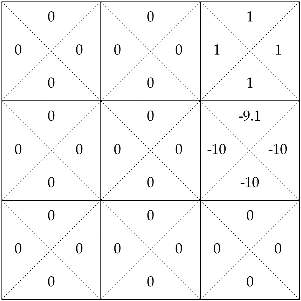
Whenever observe \((6, \uparrow),\) -10, 3:
Whenever observe \((6, \uparrow),\) -10, 2:
\(\mathrm{Q}_{\text {new }}(6, \uparrow) \leftarrow\)
\(-10 +\gamma \max _{a^{\prime}} \mathrm{Q}_{\text {old }}\left(3, a^{\prime}\right)\)
\(=-10 + 0.9 * 1 = -9.1 \)
\(\mathrm{Q}_{\text {new }}(s, a) \leftarrow ~ r +\gamma \max _{a^{\prime}} \mathrm{Q}_{\text {old }}\left(s^{\prime}, a^{\prime}\right)\)
\(\mathrm{Q}_{\text {new }}(s, a) \leftarrow ~ r +\gamma \max _{a^{\prime}} \mathrm{Q}_{\text {old }}\left(s^{\prime}, a^{\prime}\right)\)
target
\((s, a)\)
\(r \)
\(s^{\prime}\)
\(\dots\)
\((6,\uparrow)\)
-10
2
\((6,\uparrow)\)
-10
3
\((6,\uparrow)\)
-10
2
\((6,\uparrow)\)
-10
3
\(\dots\)
\bigg(
\bigg)
\alpha
- Core update rule of Q-learning
- \(\alpha \in [0, 1]:\) hyperparameter, trades off how much we trust new evidence versus old belief
- What we saw was \(\alpha = 1\): trust new experience entirely
- Let's see an example using \(\alpha = 0.7\)
😍 merge old belief and target
\alpha
\(r +\gamma \max _{a^{\prime}} \mathrm{Q}_{\text {old }}\left(s^{\prime}, a^{\prime}\right)\)
\(\mathrm{Q}_{\text {new }}(s, a) ~ \leftarrow ~ \)
\((1- \quad ) \)
\(\mathrm{Q}_{\text {old }}(s, a)\)
\(+\)
learning rate
target
old belief
\(+\)
learning rate
\((1- \qquad \qquad \qquad ) \)
\(\mathrm{Q}_\text{old}(s, a)\)
\(\mathrm{Q}_{\text{new}}(s, a)\)
\(\mathrm{Q}_{\text {new }}(s, a) \leftarrow (1-\alpha) \mathrm{Q}_{\text {old }}(s, a)+\alpha\left(r+\gamma \max _{a^{\prime}} \mathrm{Q}_{\text {old }}\left(s^{\prime}, a^{\prime}\right)\right)\)
\(\gamma = 0.9\)
\(\alpha = 0.7\)
\(\mathrm{Q}_{\text {new }}(1, \uparrow) \leftarrow (1-0.7) \mathrm{Q}_{\text {old }}(1, \uparrow)+0.7\left(0+ 0.9\max _{a^{\prime}} \mathrm{Q}_{\text {old }}\left(1, a^{\prime}\right)\right)\)
\(= (1-0.7)*0 + 0.7*( 0 + 0.9*0) = 0\)
\((s, a)\)
\(r \)
\(s^{\prime}\)
\((1,\uparrow)\)
0
1
\((3,\uparrow)\)
1
3
\((6,\uparrow)\)
-10
3
\((6,\uparrow)\)
-10
2
\((6,\uparrow)\)
-10
3
\((6,\uparrow)\)
-10
2
\((s, a)\)
\(r \)
\(s^{\prime}\)
\(\mathrm{Q}_\text{old}(s, a)\)
\(\mathrm{Q}_{\text{new}}(s, a)\)
\(\mathrm{Q}_{\text {new }}(s, a) \leftarrow (1-\alpha) \mathrm{Q}_{\text {old }}(s, a)+\alpha\left(r+\gamma \max _{a^{\prime}} \mathrm{Q}_{\text {old }}\left(s^{\prime}, a^{\prime}\right)\right)\)
\(\gamma = 0.9\)
\(\alpha = 0.7\)
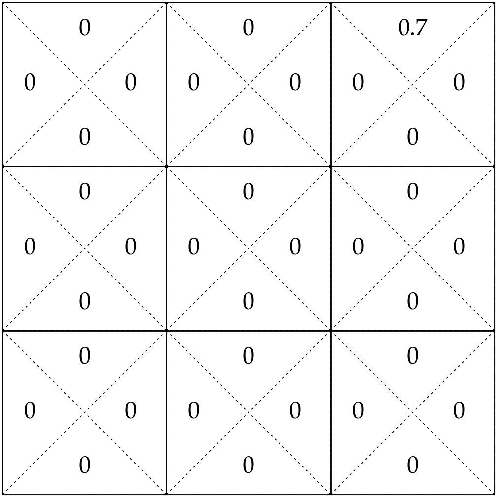
\(\mathrm{Q}_{\text {new }}(3, \uparrow) \leftarrow (1-0.7) \mathrm{Q}_{\text {old }}(3, \uparrow)+0.7\left(1+ 0.9\max _{a^{\prime}} \mathrm{Q}_{\text {old }}\left(3, a^{\prime}\right)\right)\)
\(= (1-0.7)*0 + 0.7*( 1 + 0.9*0) = 0.7\)
\((s, a)\)
\(r \)
\(s^{\prime}\)
\((1,\uparrow)\)
0
1
\((3,\uparrow)\)
1
3
\((6,\uparrow)\)
-10
3
\((6,\uparrow)\)
-10
2
\((6,\uparrow)\)
-10
3
\((6,\uparrow)\)
-10
2
\((s, a)\)
\(r \)
\(s^{\prime}\)
\(\mathrm{Q}_\text{old}(s, a)\)
\(\mathrm{Q}_{\text{new}}(s, a)\)
\(\mathrm{Q}_{\text {new }}(s, a) \leftarrow (1-\alpha) \mathrm{Q}_{\text {old }}(s, a)+\alpha\left(r+\gamma \max _{a^{\prime}} \mathrm{Q}_{\text {old }}\left(s^{\prime}, a^{\prime}\right)\right)\)
\(\alpha = 0.7\)

\(\gamma = 0.9\)
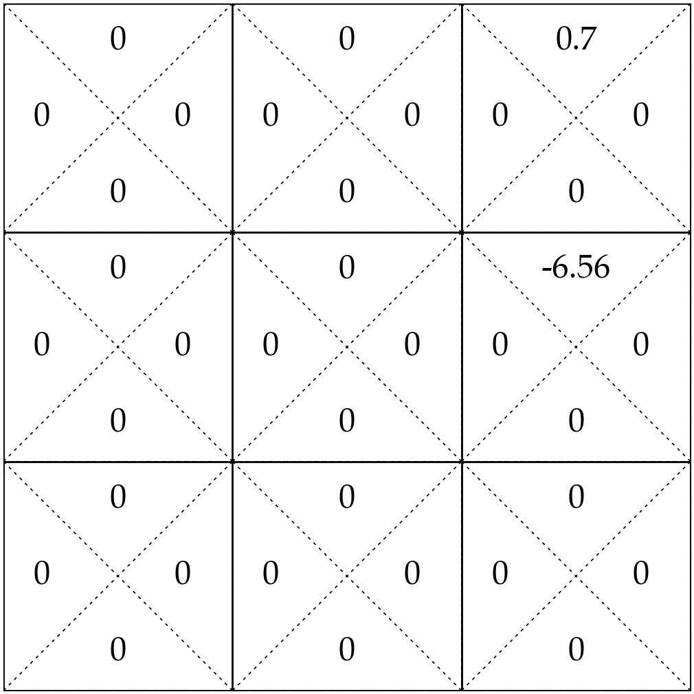
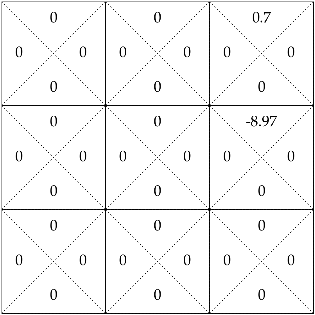
\(\mathrm{Q}_{\text {new }}(6, \uparrow) \leftarrow (1-0.7) \mathrm{Q}_{\text {old }}(6, \uparrow)+0.7\left(-10+ 0.9\max _{a^{\prime}} \mathrm{Q}_{\text {old }}\left(3, a^{\prime}\right)\right)\)
\(= (1-0.7)*0 + 0.7*( -10 + 0.9*0.7) = -6.56\)
\((s, a)\)
\(r \)
\(s^{\prime}\)
\((1,\uparrow)\)
0
1
\((3,\uparrow)\)
1
3
\((6,\uparrow)\)
-10
3
\((6,\uparrow)\)
-10
2
\((6,\uparrow)\)
-10
3
\((6,\uparrow)\)
-10
2
\((s, a)\)
\(r \)
\(s^{\prime}\)
\(\mathrm{Q}_\text{old}(s, a)\)
\(\mathrm{Q}_{\text{new}}(s, a)\)
\(\mathrm{Q}_{\text {new }}(s, a) \leftarrow (1-\alpha) \mathrm{Q}_{\text {old }}(s, a)+\alpha\left(r+\gamma \max _{a^{\prime}} \mathrm{Q}_{\text {old }}\left(s^{\prime}, a^{\prime}\right)\right)\)
\(\gamma = 0.9\)
\(\alpha = 0.7\)
\(\mathrm{Q}_{\text {new }}(6, \uparrow) \leftarrow (1-0.7) \mathrm{Q}_{\text {old }}(6, \uparrow)+0.7\left(-10+ 0.9\max _{a^{\prime}} \mathrm{Q}_{\text {old }}\left(2, a^{\prime}\right)\right)\)
\(= (1-0.7)*-6.56 + 0.7*( -10 + 0.9*0) = -8.97\)
\((s, a)\)
\(r \)
\(s^{\prime}\)
\((1,\uparrow)\)
0
1
\((3,\uparrow)\)
1
3
\((6,\uparrow)\)
-10
3
\((6,\uparrow)\)
-10
2
\((6,\uparrow)\)
-10
3
\((6,\uparrow)\)
-10
2
\((s, a)\)
\(r \)
\(s^{\prime}\)
\(\mathrm{Q}_\text{old}(s, a)\)
\(\mathrm{Q}_{\text{new}}(s, a)\)
\(\mathrm{Q}_{\text {new }}(s, a) \leftarrow (1-\alpha) \mathrm{Q}_{\text {old }}(s, a)+\alpha\left(r+\gamma \max _{a^{\prime}} \mathrm{Q}_{\text {old }}\left(s^{\prime}, a^{\prime}\right)\right)\)
\(\gamma = 0.9\)
\(\alpha = 0.7\)
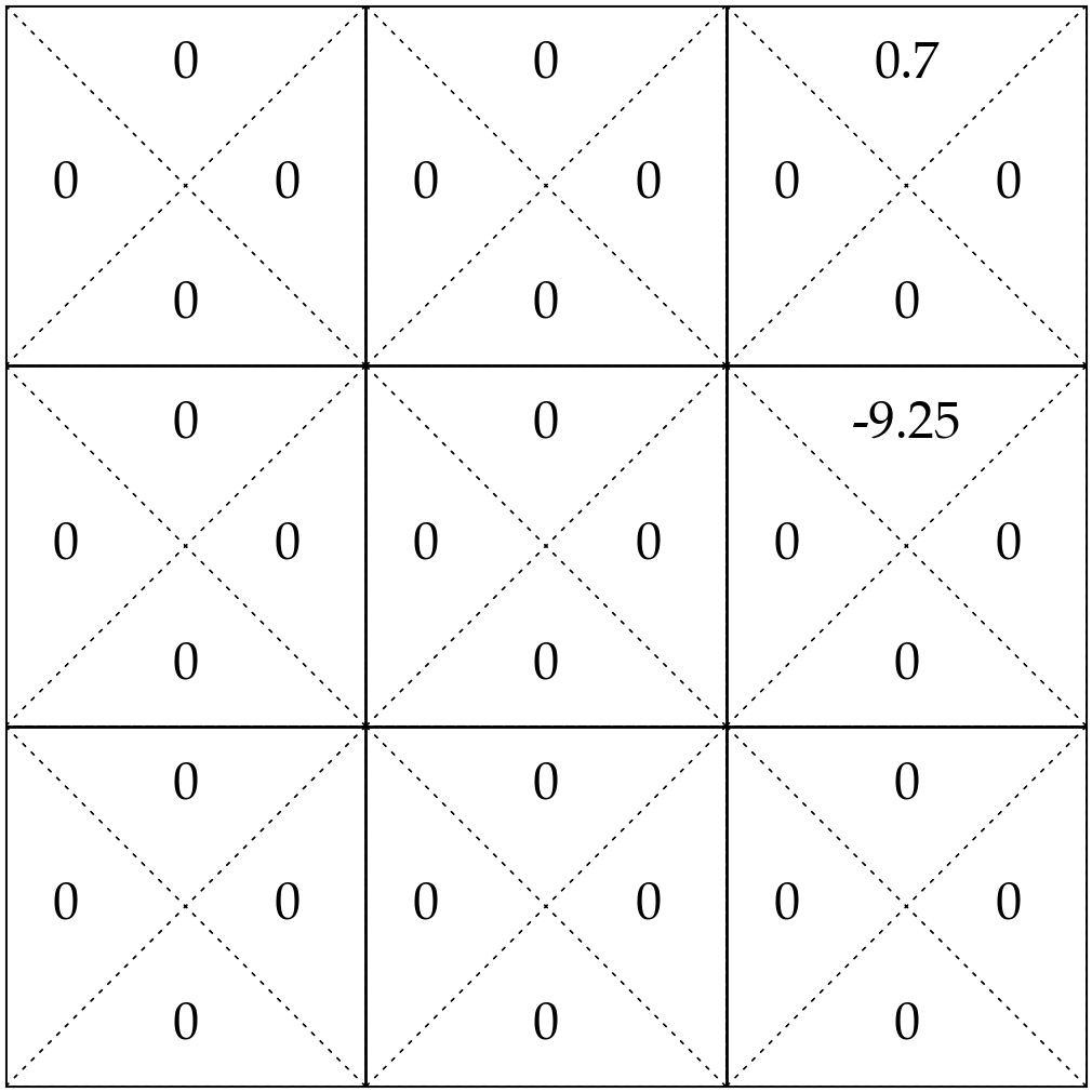
\(\mathrm{Q}_{\text {new }}(6, \uparrow) \leftarrow (1-0.7) \mathrm{Q}_{\text {old }}(6, \uparrow)+0.7\left(-10+ 0.9\max _{a^{\prime}} \mathrm{Q}_{\text {old }}\left(3, a^{\prime}\right)\right)\)
\(= (1-0.7)*-8.97 + 0.7*( -10 + 0.9*0.7) = -9.25\)
\((s, a)\)
\(r \)
\(s^{\prime}\)
\((1,\uparrow)\)
0
1
\((3,\uparrow)\)
1
3
\((6,\uparrow)\)
-10
3
\((6,\uparrow)\)
-10
2
\((6,\uparrow)\)
-10
3
\((6,\uparrow)\)
-10
2
\((s, a)\)
\(r \)
\(s^{\prime}\)
\(\mathrm{Q}_\text{old}(s, a)\)
\(\mathrm{Q}_{\text{new}}(s, a)\)
\(\mathrm{Q}_{\text {new }}(s, a) \leftarrow (1-\alpha) \mathrm{Q}_{\text {old }}(s, a)+\alpha\left(r+\gamma \max _{a^{\prime}} \mathrm{Q}_{\text {old }}\left(s^{\prime}, a^{\prime}\right)\right)\)
\(\gamma = 0.9\)
\(\alpha = 0.7\)
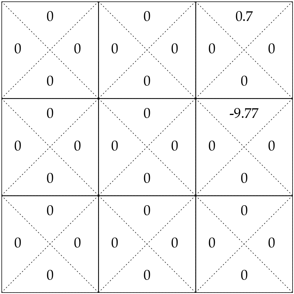
\(\mathrm{Q}_{\text {new }}(6, \uparrow) \leftarrow (1-0.7) \mathrm{Q}_{\text {old }}(6, \uparrow)+0.7\left(-10+ 0.9\max _{a^{\prime}} \mathrm{Q}_{\text {old }}\left(2, a^{\prime}\right)\right)\)
\(= (1-0.7)*-9.25 + 0.7*( -10 + 0.9*0) = -9.77\)
\((s, a)\)
\(r \)
\(s^{\prime}\)
\((1,\uparrow)\)
0
1
\((3,\uparrow)\)
1
3
\((6,\uparrow)\)
-10
3
\((6,\uparrow)\)
-10
2
\((6,\uparrow)\)
-10
3
\((6,\uparrow)\)
-10
2
\((s, a)\)
\(r \)
\(s^{\prime}\)
- To update a particular Q(s, a), we need experience from actually taking that \(a\) in that \(s\).
- If we never try a move, its Q-value never changes.
- So if we have one play left, which \((s,a)\) should we try?
\(\mathrm{Q}_{\text {new }}(s, a) \leftarrow (1-\alpha) \mathrm{Q}_{\text {old }}(s, a)+\alpha\left(r+\gamma \max _{a^{\prime}} \mathrm{Q}_{\text {old }}\left(s^{\prime}, a^{\prime}\right)\right)\)
Depends on
- are we trying to "win" the game, or
- are we trying to get more accurate Q estimates
This is the fundamental dilemma in reinforcement learning... and in life!
Whether to exploit what we've already learned or explore to discover something better.
Exploration has real costs: A/B tests give real users bad experiences, medical trials risk patient safety, self-driving cars risk lives.

Seinfeld, S06E09
[feynmanlectures.caltech.edu]
- with probability \(\epsilon\), choose an action \(a \in \mathcal{A}\) uniformly at random
\(\epsilon\) trades off exploration versus exploitation.
During learning, especially in early stages, we'd like to explore and observe diverse \((s,a\)) consequences.
During later stages, we can act more greedily w.r.t. the current estimated Q values
\(\epsilon\)-greedy action selection strategy
- with probability \((1-\epsilon)\), choose \(\arg \max _{\mathrm{a}} \mathrm{Q}_{\text{old}}(s, \mathrm{a})\)
- for \(s \in \mathcal{S}, a \in \mathcal{A}\) :
- \(\mathrm{Q}_{\text {old }}(\mathrm{s}, \mathrm{a})=0\)
- while True:
- for \(s \in \mathcal{S}, a \in \mathcal{A}\) :
- \(\mathrm{Q}_{\text {new }}(s, a) \leftarrow \mathrm{R}(s, a)+\gamma \sum_{s^{\prime}} \mathrm{T}\left(s, a, s^{\prime}\right) \max _{a^{\prime}} \mathrm{Q}_{\text {old }}\left(s^{\prime}, a^{\prime}\right)\)
- if \(\max _{s, a}\left|Q_{\text {old }}(s, a)-Q_{\text {new }}(s, a)\right|<\epsilon:\)
- return \(\mathrm{Q}_{\text {new }}\)
- \(\mathrm{Q}_{\text {old }} \leftarrow \mathrm{Q}_{\text {new }}\)
Value Iteration\((\mathcal{S}, \mathcal{A}, \mathrm{T}, \mathrm{R}, \gamma, \epsilon)\)
"calculating"
"learning" (estimating)
Q-Learning \(\left(\mathcal{S}, \mathcal{A}, \gamma, \alpha, s_0,\right. \text{max-iter})\)
1. \(i=0\)
2. for \(s \in \mathcal{S}, a \in \mathcal{A}:\)
3. \({\mathrm{Q}_\text{old}}(s, a) = 0\)
4. \(s \leftarrow s_0\)
5. while \(i < \text{max-iter}:\)
6. \(a \gets \text{select}\_\text{action}(s, {\mathrm{Q}_\text{old}}(s, a))\)
7. \(r,s' \gets \text{execute}(a)\)
8. \({\mathrm{Q}}_{\text{new}}(s, a) \leftarrow (1-\alpha){\mathrm{Q}}_{\text{old}}(s, a) + \alpha(r + \gamma \max_{a'}{\mathrm{Q}}_{\text{old}}(s', a'))\)
9. \(s \leftarrow s'\)
10. \(i \leftarrow (i+1)\)
11. \(\mathrm{Q}_{\text{old}} \leftarrow \mathrm{Q}_{\text{new}}\)
12. return \(\mathrm{Q}_{\text{new}}\)
"learning"
Q-Learning \(\left(\mathcal{S}, \mathcal{A}, \gamma, \alpha, s_0,\right. \text{max-iter})\)
1. \(i=0\)
2. for \(s \in \mathcal{S}, a \in \mathcal{A}:\)
3. \({\mathrm{Q}_\text{old}}(s, a) = 0\)
4. \(s \leftarrow s_0\)
5. while \(i < \text{max-iter}:\)
6. \(a \gets \text{select}\_\text{action}(s, {\mathrm{Q}_\text{old}}(s, a))\)
7. \(r,s' \gets \text{execute}(a)\)
8. \({\mathrm{Q}}_{\text{new}}(s, a) \leftarrow (1-\alpha){\mathrm{Q}}_{\text{old}}(s, a) + \alpha(r + \gamma \max_{a'}{\mathrm{Q}}_{\text{old}}(s', a'))\)
9. \(s \leftarrow s'\)
10. \(i \leftarrow (i+1)\)
11. \(\mathrm{Q}_{\text{old}} \leftarrow \mathrm{Q}_{\text{new}}\)
12. return \(\mathrm{Q}_{\text{new}}\)
- Remarkably, 👈 can converge to the true \(\mathrm{Q}^*_{\infty}\)
\(^1\) given that we visit all \(s,a\) infinitely often, and satisfy a decaying condition on the learning rate \(\alpha\).
- Once converged, act greedily w.r.t \(\mathrm{Q}^*\) again.
- But convergence can be extremely slow, and often not practical.
- Three hyperparameters :
- discount factor \(\gamma\)
- learning rate \(\alpha\)
- exploration rate \(\epsilon\)
all between 0 and 1
each controls some trade-off
Outline
- Reinforcement learning setup
- Tabular Q-learning
- exploration vs. exploitation
- \(\epsilon\)-greedy action selection
- Fitted Q-learning
- (Policy gradient)
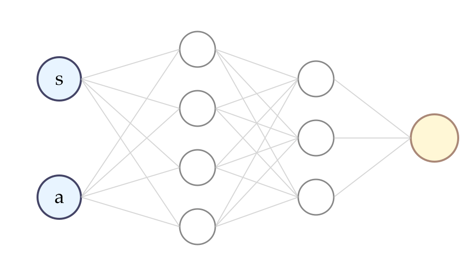
- So far, Q-learning is sensible for the (small) tabular setting.
- What if \(\mathcal{S}\) and/or \(\mathcal{A}\) are large, or even continuous?
- We can't keep a table; we must approximate \(\mathrm{Q}(s,a)\) with a function \(\mathrm{Q}_{\theta}(s,a).\)
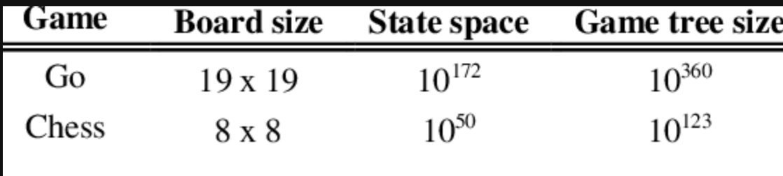
Continuous state and action space
\(10^{16992}\) (pixels) states
Fitted Q-learning: from table to functions
- Notice that the core update rule of Q-learning:
is equivalent to:
\(\mathrm{Q}_{\text {new}}(s, a) \leftarrow\mathrm{Q}_{\text {old }}(s, a)+\alpha\left([r+\gamma \max _{a^{\prime}} \mathrm{Q}_{\text {old}}(s', a')] - \mathrm{Q}_{\text {old }}(s, a)\right)\)
new belief
\(\leftarrow\)
old belief
learning rate
+
(
target
-
old belief
)
\mathrm{Q}_{\text {new }}(s, a) \leftarrow(1-\alpha) \mathrm{Q}_{\text {old }}(s, a)+\alpha\left(r+\gamma \max _{a^{\prime}} \mathrm{Q}_{\text {old }}\left(s^{\prime}, a^{\prime}\right)\right)
Gradient update rule when minimizing \((\text{target} - \text{guess}_{\theta})^2\)
\(\theta_{\text{new}} \leftarrow \theta_{\text{old}} + \eta (\text{target} - \text{guess}_{\theta})\nabla_{\theta}\text{guess}\)
- Does this
- Yes! Recall:
remind you of something?
\(\mathrm{Q}_{\text {new}}(s, a) \leftarrow\mathrm{Q}_{\text {old }}(s, a)+\alpha\left([r+\gamma \max _{a^{\prime}} \mathrm{Q}_{\text {old}}(s', a')] - \mathrm{Q}_{\text {old }}(s, a)\right)\)
new belief
\(\leftarrow\)
old belief
learning rate
+
(
target
-
old belief
)
- Generalize tabular Q-learning for continuous state/action space:
\(\left(\text{target} -\mathrm{Q}_{\theta}(s, a)\right)^2\)
- parameterize \(\mathrm{Q}_{\theta}(s,a)\)
- execute \((s,a),\) observe\((r, s'),\) construct the target
- regress \(\mathrm{Q}_{\theta}(s,a)\) against the target, i.e. update \(\theta\) via gradient-descent to minimize
\(r+\gamma \max _{a^{\prime}} \mathrm{Q}_{\theta}\left(s^{\prime}, a^{\prime}\right)\)
- Same idea as before — we adjust our belief toward a target.
- Now Q is a function (e.g. a neural network) and \(\theta\) are its weights.
From table to functions
tabular: a lookup, one entry per \((s, a)\)
⟹
scale up:
large/continuous \(\mathcal{S}\), \(\mathcal{A}\)
fitted: any \((s,a)\) goes through one shared \(\theta\)
Updating one \((s, a)\) now nudges \(\theta\), which changes \(Q_\theta\) at nearby \((s, a)\) too.
The function generalizes; the table doesn't.
\(\mathrm{Q}_\theta\)
Fitted Q-learning: the training loop
1. Sample experience
interact: observe \((s, a, r, s')\)
2. Build target
\(y = r + \gamma \max_{a'} \mathrm{Q}_\theta(s', a')\)
3. Compute loss
\(\mathcal{L} = (y - \mathrm{Q}_\theta(s, a))^2\)
4. Gradient step
\(\theta \leftarrow \theta - \eta \nabla_\theta \mathcal{L}\)
repeat
Same shape as supervised learning; except the “label” \(y\) is built from our own current estimate. (Bootstrapping.)
Outline
- Reinforcement learning setup
- Tabular Q-learning
- exploration vs. exploitation
- \(\epsilon\)-greedy action selection
- Fitted Q-learning
- (Policy gradient)
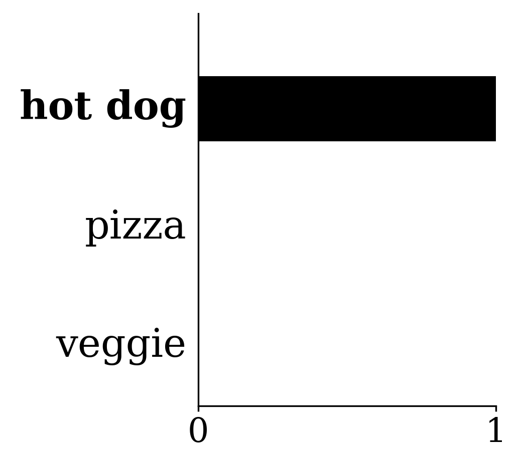
🌭
\xrightarrow{\,h_\theta\,}
y \text{ (true label)}
= [1,\; 0,\; 0]
current prediction \(g=\text{softmax}(\cdot)\)
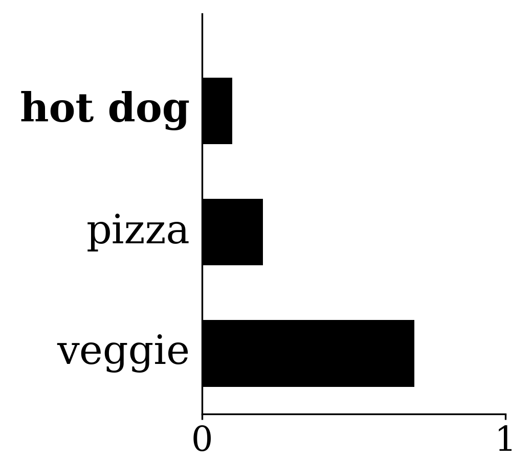
= [0.1,\; 0.2,\; 0.7]
\xrightarrow{\;-\log\;}
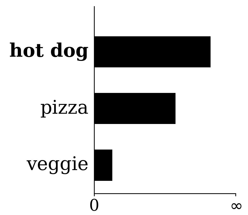
-\!\log(g)
\approx [2.30,\; 1.61,\; 0.36]
\odot
\mathcal{L}_{\mathrm{nllm}} = -\sum_{k} y_k \cdot \log(g_k)
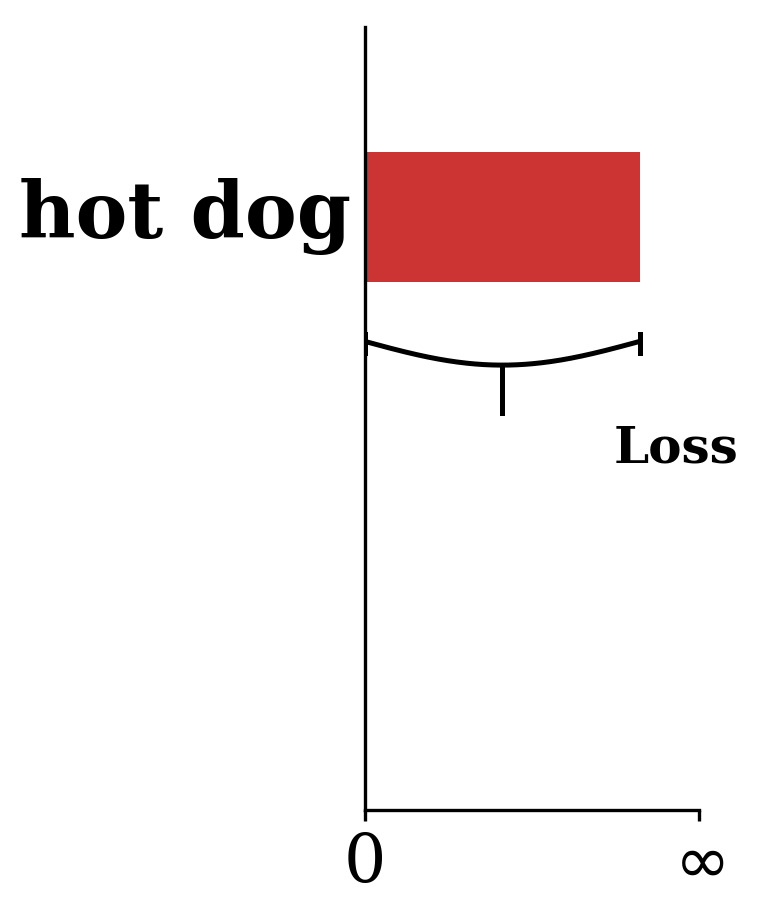
\text{Loss} \approx 2.30
To reduce the loss, \(\theta\) needs to change so \(g_{\text{hotdog}}\) can go up.
This signal (from the true label \(y\)) backprop to \(\theta\) through \(-\!\log\) and softmax, so we can optimize via gradient descent.
Recall:

🤷 ↑ ? ↓
[image edited from: Andrej Karpathy]
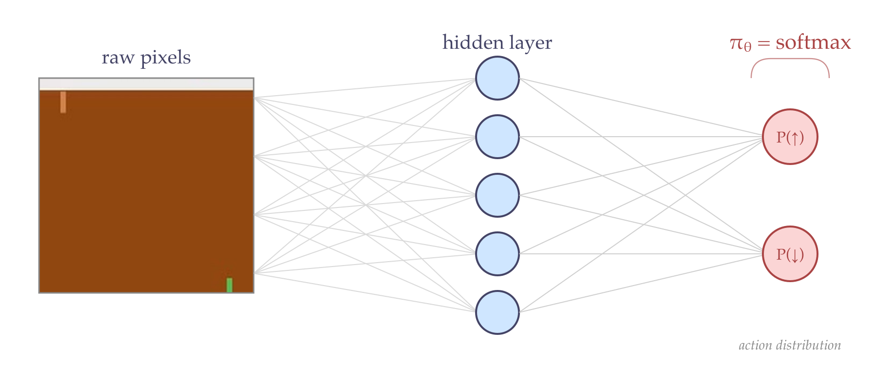
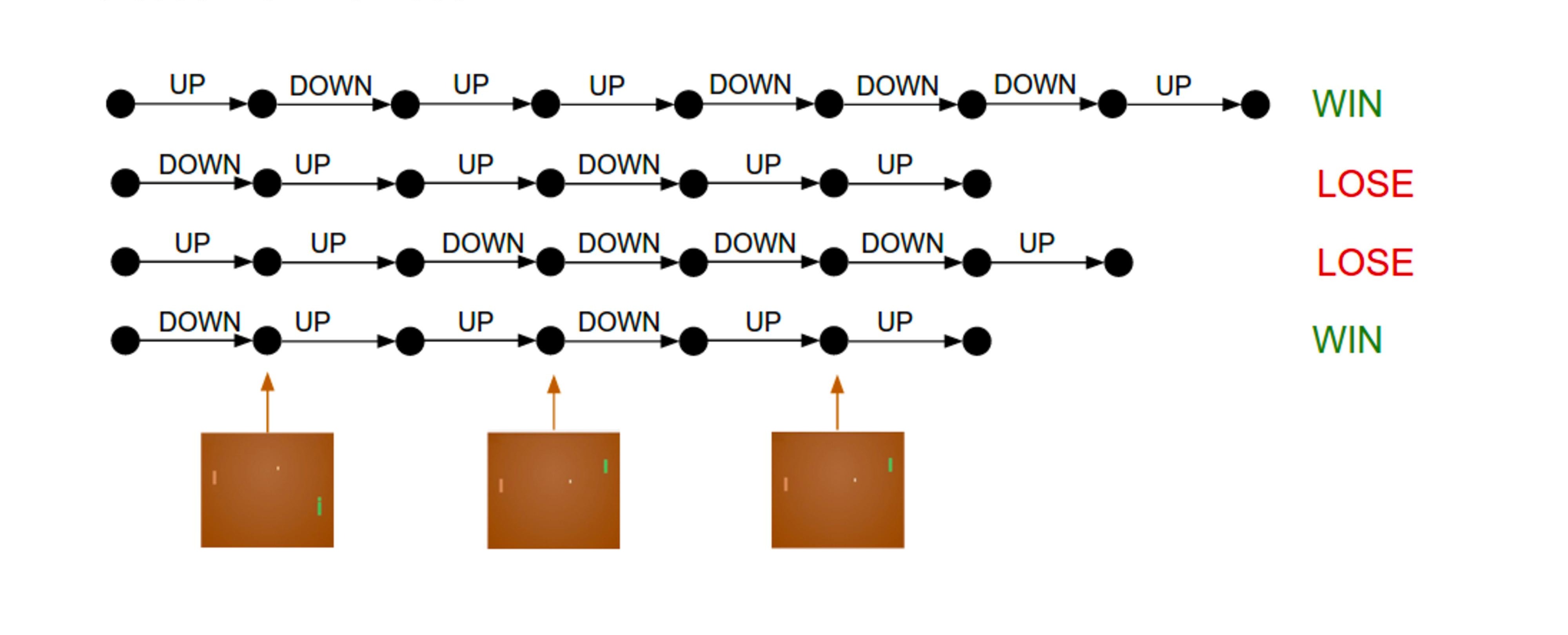
2. Run \(\pi_\theta\) for a while. Keep track of the return.
Policy gradients:
1. Parametrize the policy \(\pi\) with \(\theta.\)
3. Update \(\theta\) so "good" trajectories more likely to happen.
Made rigorous by the log-derivative trick (REINFORCE). We will skip the derivation.
\(\nabla_\theta \mathrm{J}(\theta) \;=\; \mathbb{E}_{\tau \sim \pi_\theta}\!\left[\sum_{t}\right.\) \(\nabla_\theta \log \pi_\theta(a_t \mid s_t)\) \(\cdot\) \(\mathrm{R}(\tau)\) \(\left.\right]\)
trajectory drawn under the current policy
sum over timesteps
push \(\theta\) to make the taken action more likely
weight by how good the trajectory was
Sample trajectories, observe returns, nudge \(\theta\) to make actions in good trajectories more likely.
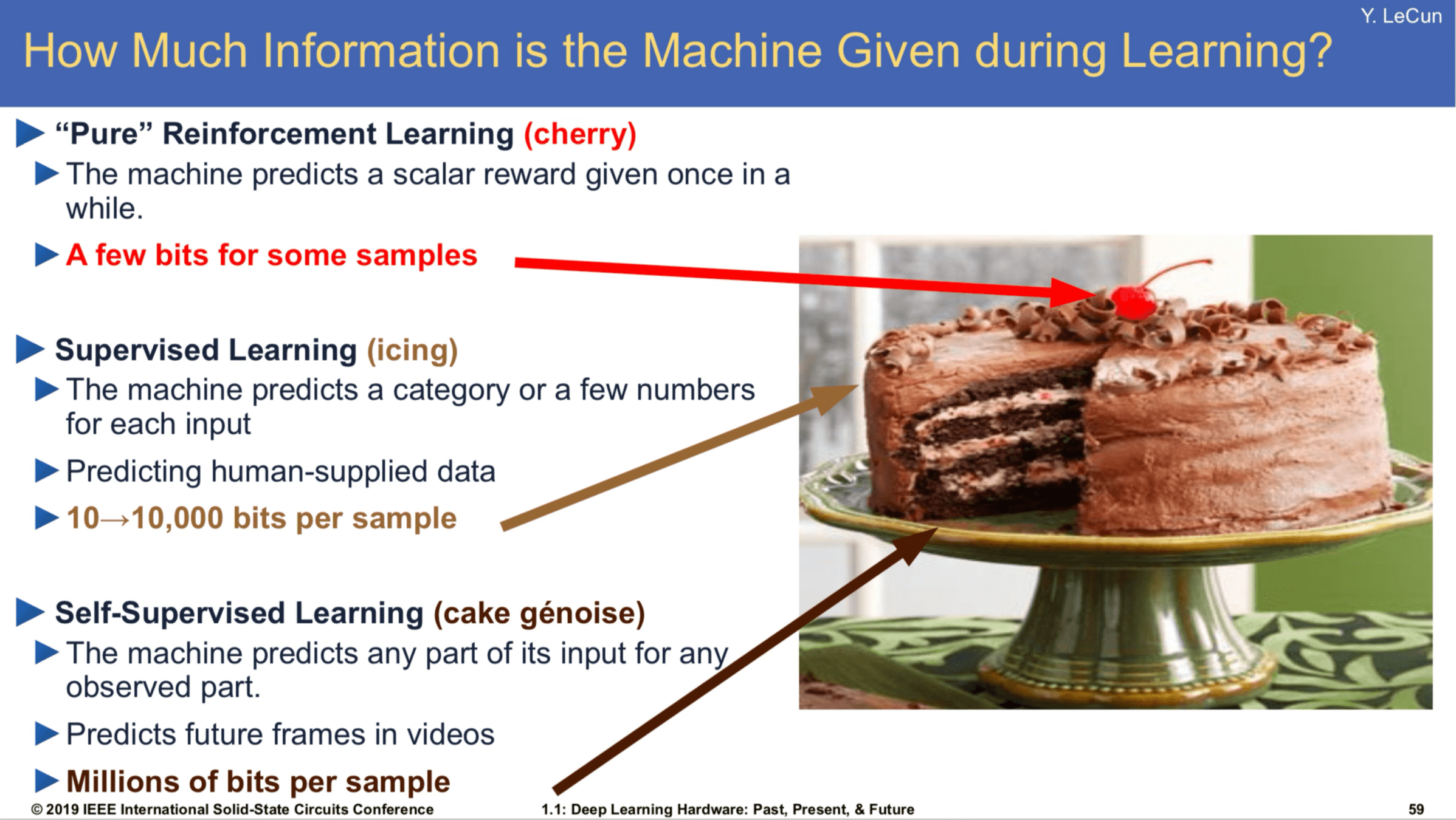
[Slide Credit: Yann LeCun]
Summary
- Last week: find good policies in a known MDP (high cumulative expected reward).
- In RL, the transitions and rewards are unknown. We still want a good policy; we get one by estimating Q.
- Exploration vs. exploitation: choose actions to gain reward while still learning.
- Q-learning converges to \(\mathrm{Q}^*\) (with enough exploration).
- Deep Q-learning extends to large or continuous state spaces by parameterizing Q.
6.390 IntroML (Spring 26) - Lecture 11 Reinforcement Learning
By Shen Shen


