[Image credit: SDXL: Improving Latent Diffusion Models for High-Resolution Image Synthesis https://arxiv.org/pdf/2307.01952]

Text-to-image generation

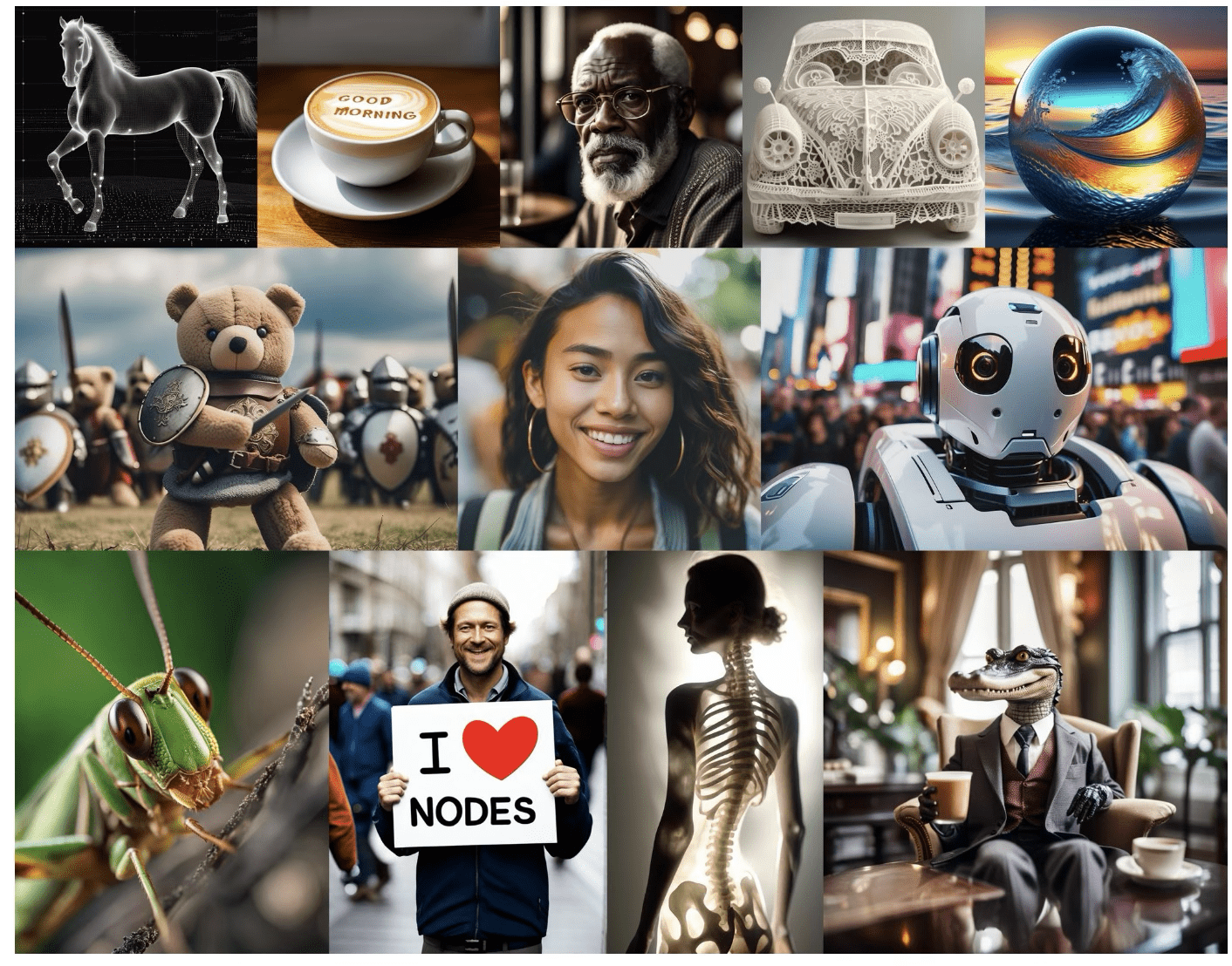
Image credit: https://github.com/CompVis/stable-diffusion

Sketch-to-Image: coarse-grained control

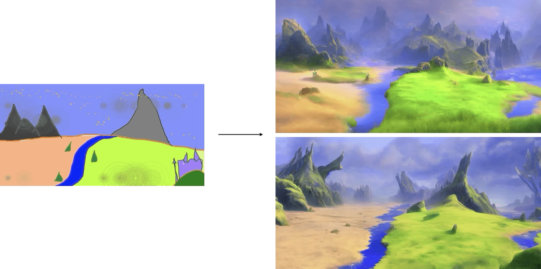
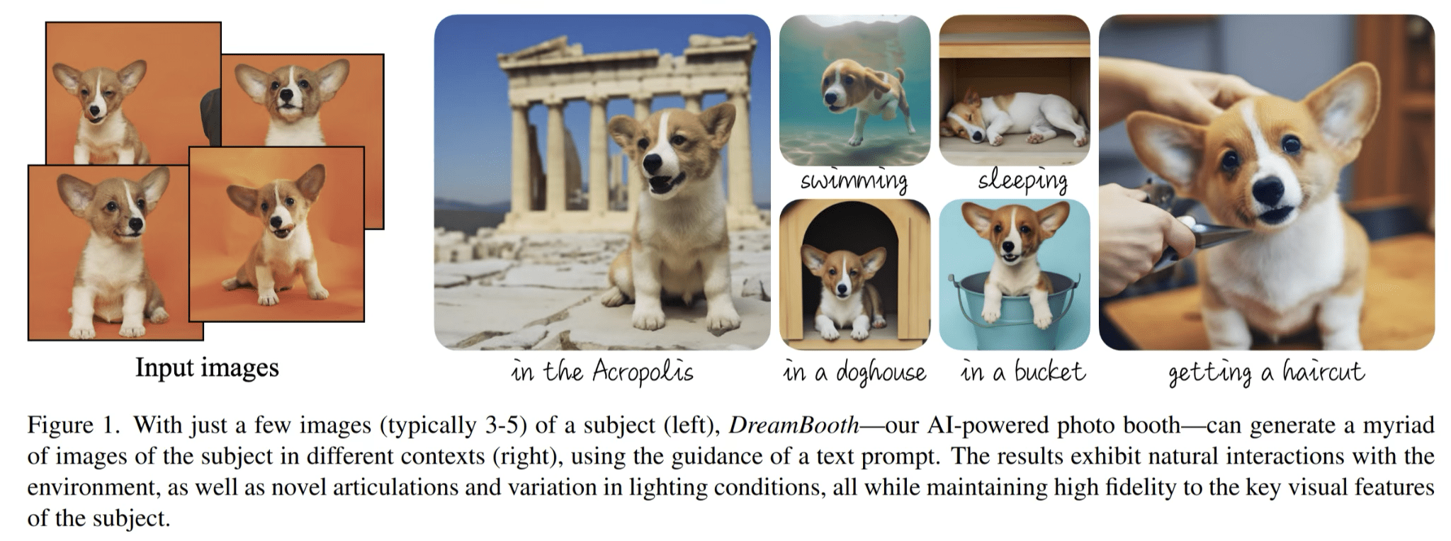
Image credit: DreamBooth: Fine Tuning Text-to-Image Diffusion Models for Subject-Driven Generation https://arxiv.org/pdf/2208.12242

Image editing and composition

Diffusion “prior” for image restoration

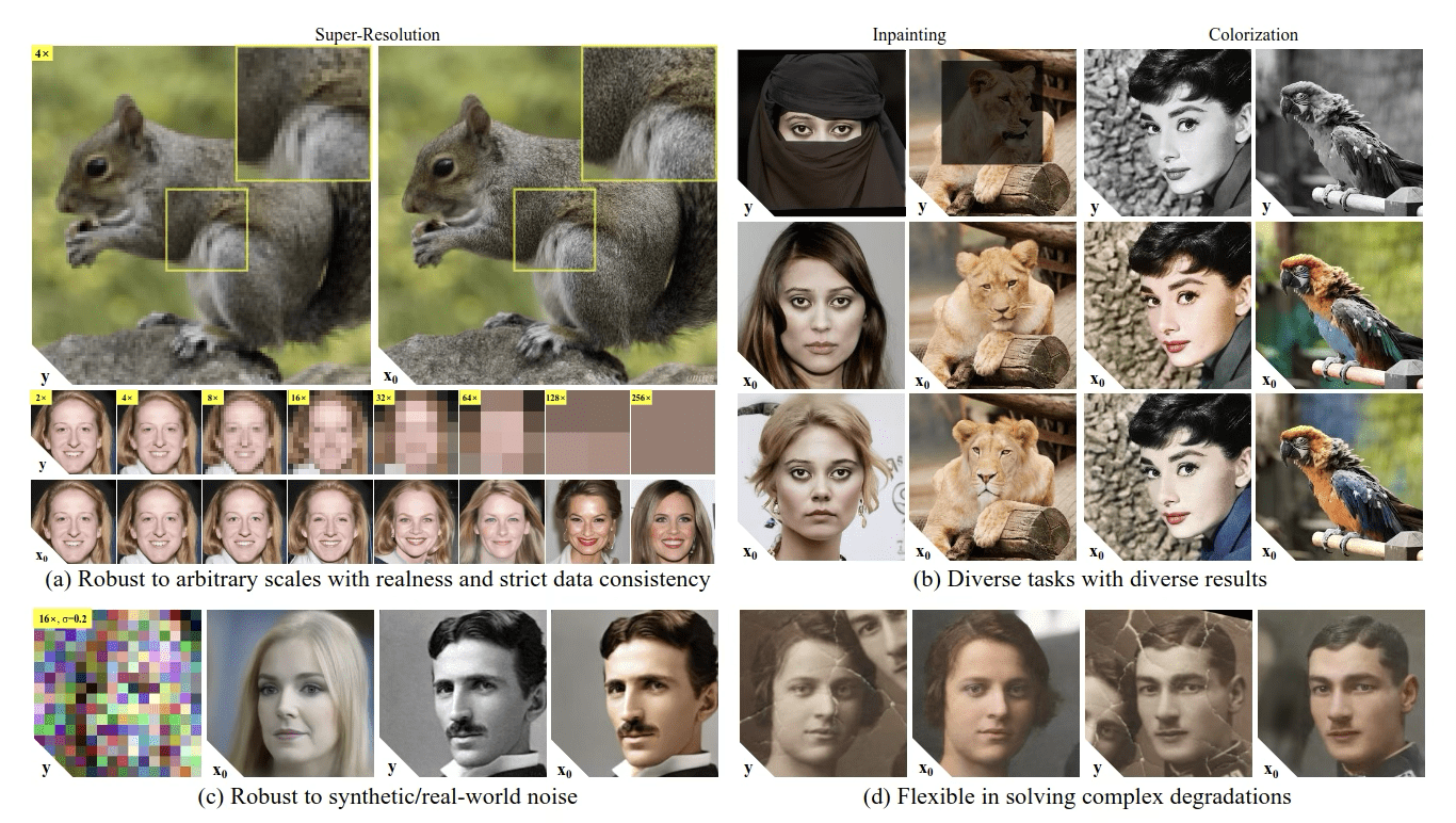
Image credit: Zero-Shot Image Restoration Using Denoising Diffusion Null-Space Model https://arxiv.org/pdf/2212.00490

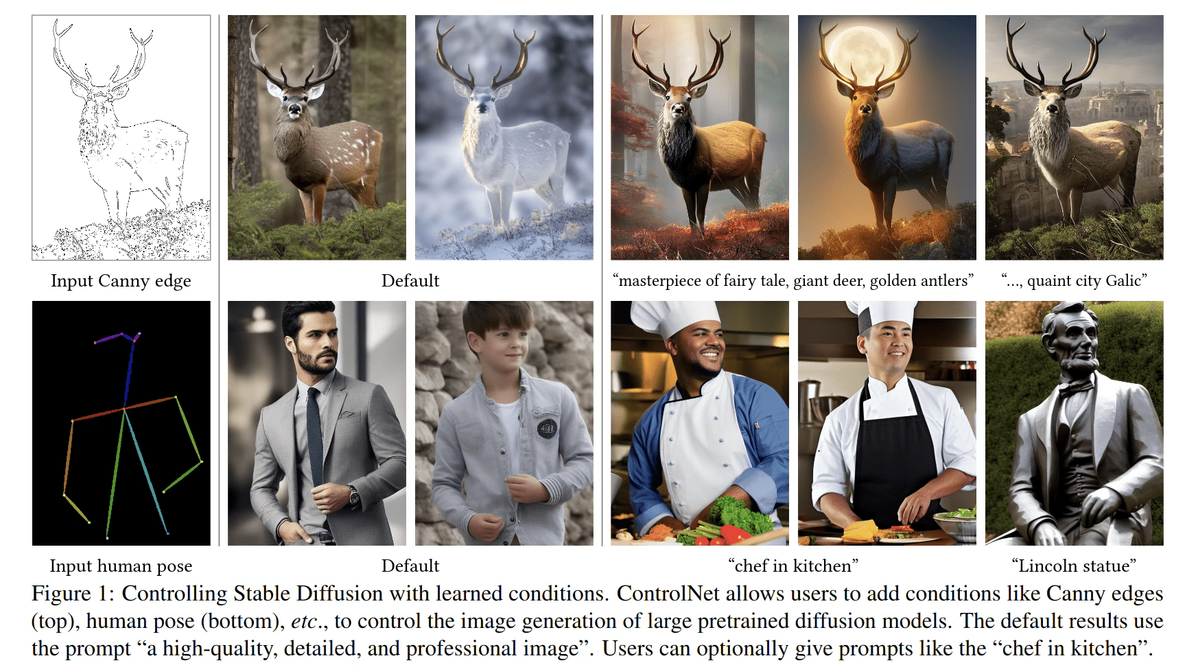
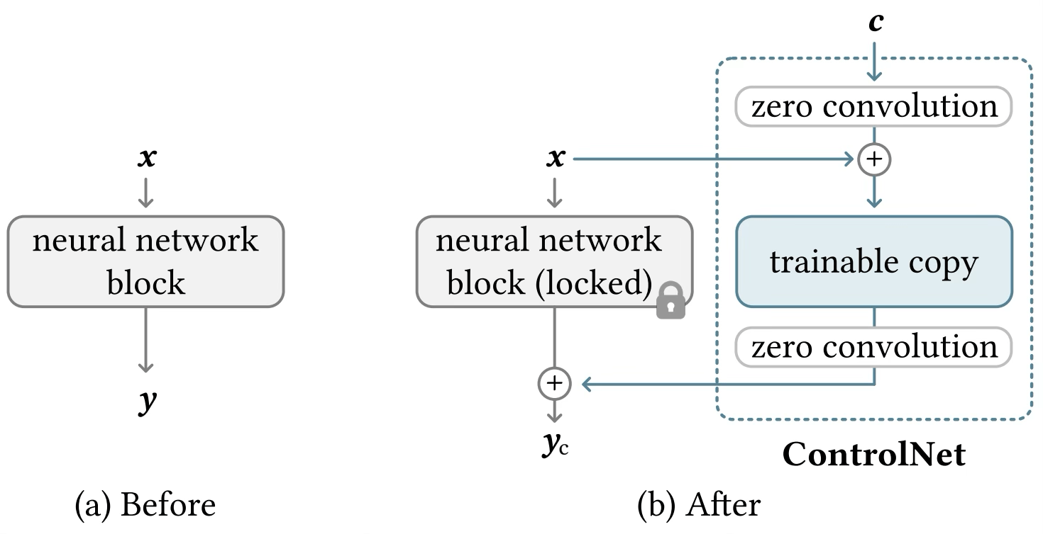
Image credit: Adding Conditional Control to Text-to-Image Diffusion Models https://arxiv.org/pdf/2302.05543

ControlNet: refined control

Text-to-audio generation 

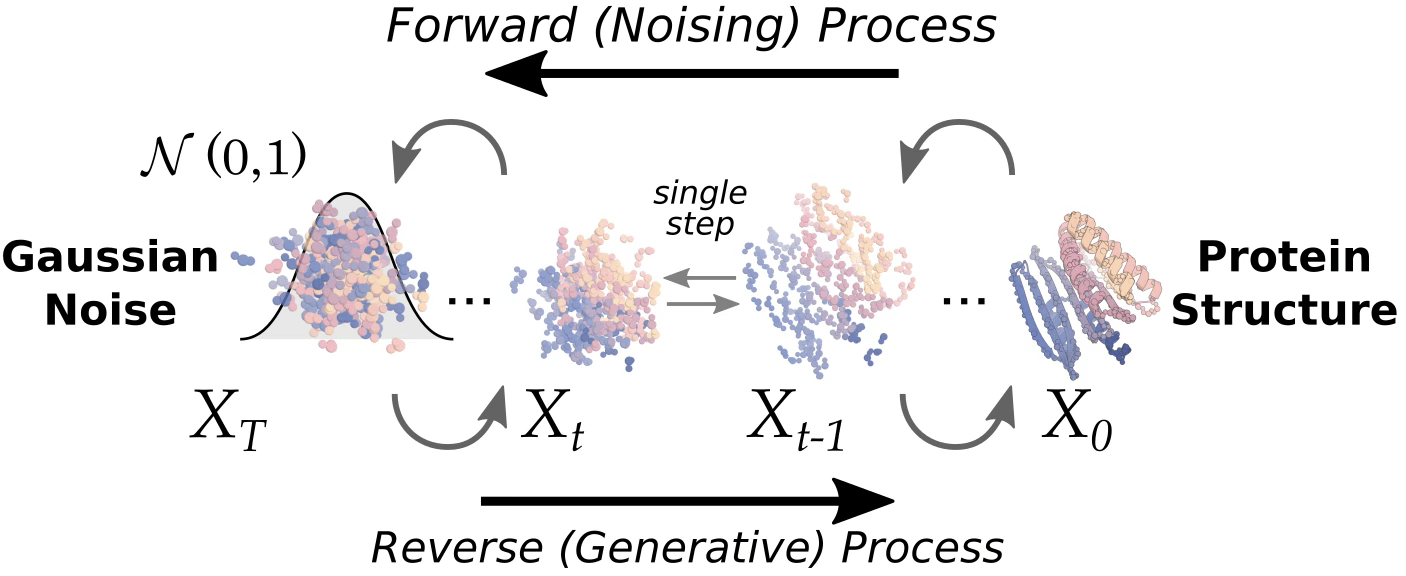
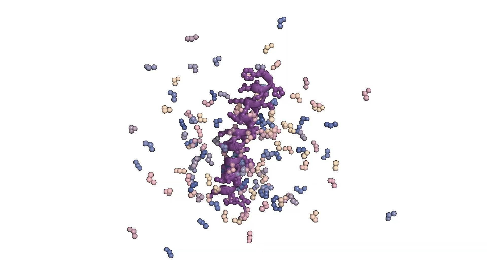
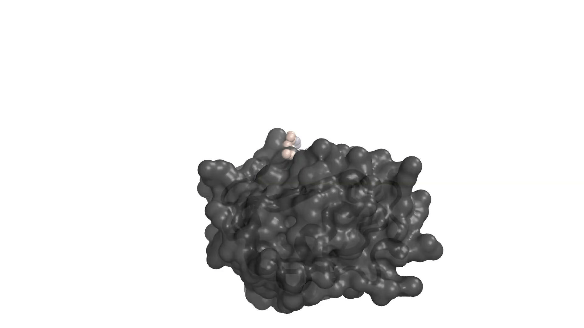
Image/video credit: RFDiffusion https://www.bakerlab.org

Key Idea: denoising in many small steps is easier than attempting to remove all noise in a single step

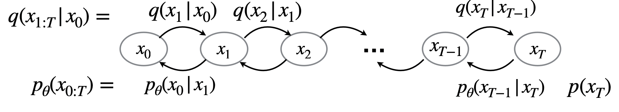
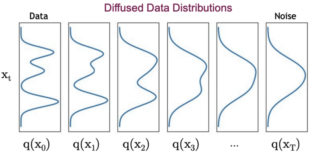
1. Forward Process

• Encoder is a fixed noising procedure \( q(x_t \mid x_{t-1}) \) which gradually adds noise to the clean data \( x_0 \), producing gradually noisy latent variables \( x_1, \dots, x_T \).

2. Backward Process

• A learned decoder \( p_\theta(x_{t-1} \mid x_t) \) aims to reverse the forward process, and reconstruct step by step moving from \( x_T \) back to \( x_0 \).
• During training, we optimize \( \theta \) so each reverse step approximates the true posterior \( q(x_{t-1} \mid x_t) \).
• At inference time, we start from pure noise \( x_T \sim \mathcal{N}(0, I) \) and apply this backward chain to generate samples.

For fixed \( \{\beta_t\}_{t \in [T]} \in (0, 1) \), let \[ q(x_t \mid x_{t-1}) := \mathcal{N}(x_t \mid \sqrt{1 - \beta_t} \, x_{t-1}, \beta_t I) \]

Equivalently, \[ x_t = \sqrt{1 - \beta_t} \, x_{t-1} + \sqrt{\beta_t} \, \epsilon, \quad \epsilon \sim \mathcal{N}(0, I) \]

\[ \Rightarrow \quad x_t = \sqrt{\bar{\alpha}_t} \, x_0 + \sqrt{1 - \bar{\alpha}_t} \, \epsilon, \quad \epsilon \sim \mathcal{N}(0, I) \]

\(\alpha_t=1-\beta_t, \quad \bar{\alpha}_t=\prod_{s=1}^t \alpha_s\)

can think of \(\sqrt{\beta_t} \approx \sigma_t-\sigma_{t-1}\) noise schedule difference

Fact:

• for small \(\beta, \exists \mu\left(x_0, x_t\right)\), s.t. \(q\left(x_{t-1} \mid x_t\right) \approx \mathcal{N}\left(x_{t-1} ; \mu\left(x_0, x_t\right), \beta_t I\right)\)
• for large \(T, q\left(x_T\right) \approx \mathcal{N}(0,1)\)

\(\alpha_t=1-\beta_t, \quad \bar{\alpha}_t=\prod_{s=1}^t \alpha_s\)

can think of \(\sqrt{\beta_t} \approx \sigma_t-\sigma_{t-1}\) noise schedule difference

Fact:

• for small \(\beta, \exists \mu\left(x_0, x_t\right)\), s.t. \(q\left(x_{t-1} \mid x_t\right) \approx \mathcal{N}\left(x_{t-1} ; \mu\left(x_0, x_t\right), \beta_t I\right)\)
• for large \(T, q\left(x_T\right) \approx \mathcal{N}(0,1)\)

\(q\left(x_{0: T}\right)=q\left(x_0\right) q\left(x_{1: T} \mid x_0\right)\)

\(=q\left(x_T\right) \prod_{t=1}^T q\left(x_{t-1} \mid x_t\right)\)

\(\approx \mathcal{N}(0, I) \prod_{t=1}^T \mathcal{N}\left(x_{t-1} ; \mu\left(x_0, x_t\right), \beta_t I\right)\)

by Markov

by the two facts

Choose to parameterize \(p_\theta\left(x_{t-1} \mid x_t\right)=\mathcal{N}\left(x_{t-1} ; \mu\left(x_0, x_t\right), \beta_t I\right)\), learn \(\hat{x}_0\left(x_t, t\right)\)

Exactly like a VAE.

There are two important variations to this training procedure:

• How noise is added (variance preserving/exploding)
• What quantity to predict (noise, data, …)

Re-parameterize:

\(x_t=x_0+\sigma_t \epsilon, \epsilon \sim \mathcal{N}(0, I)\)

\(x_0=z_0, \quad x_t=z_t / \sqrt{\bar{\alpha}_t}, \quad \sigma_t=\sqrt{\frac{1-\bar{\alpha}_t}{\bar{\alpha}_t}}\)

Re-parameterize variation tends to perform better in practice, keeps model input constant norm

Denoising diffusion models estimate a noise vector \(\epsilon\) \(\in \mathbb{R}^n\) from a given noise level \(\sigma > 0\) and noisy input \(x_\sigma \in \mathbb{R}^n\) such that for some \(x_0\) in the data manifold \(\mathcal{K}\),

\[ {x_\sigma} \;\approx\; \textcolor{green}{x_0} \;+\; \textcolor{orange}{\sigma}\, \textcolor{red}{\epsilon}. \]

A denoiser \(\textcolor{red}{\epsilon_\theta} : \mathbb{R}^n \times \mathbb{R}_+ \to \mathbb{R}^n\) is learned by minimizing

\[ L(\theta) := \mathbb{E}_{\textcolor{green}{x_0},\textcolor{orange}{\sigma},\textcolor{red}{\epsilon}} \Biggl[\Biggl\|\textcolor{red}{\epsilon_\theta}\Biggl(\textcolor{green}{x_0} + \textcolor{orange}{\sigma}\,\textcolor{red}{\epsilon}, \textcolor{orange}{\sigma}\Biggr) - \textcolor{red}{\epsilon}\Biggr\|^2\Biggr]. \]

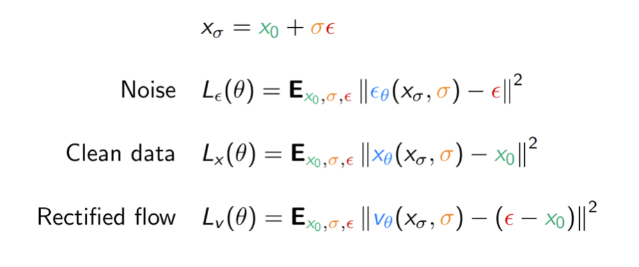
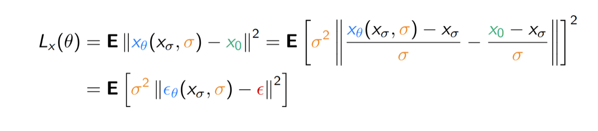
Mathematically equivalent for fixed \(\sigma\), but reweighs loss by a function of \(\sigma\) !

Score matching

Then the following holds \(\epsilon_\theta\left(x_t, t\right) \propto-\nabla_{x_t} \log q_t\left(x_t\right)\). (tweedies formula)

\(\hat{x}_0=\frac{1}{\sqrt{\bar{\alpha}_t}}\left(x_t-\sqrt{1-\bar{\alpha}_t} \hat{\epsilon}\right)\)

Can learn score instead (see hyvarinen score matching)

Let \(q_t\left(x_t\right)\) denote the marginal of \(x_t\)

\(x_{t-1}=\underbrace{\frac{1}{\alpha_t}\left(x_t-\frac{\beta_t}{1-\alpha_t} \epsilon_\theta\left(x_t, t\right)\right)}_{\mu_t}+\underbrace{\beta_t}_{\text {noise scale }} z\).

\(x_{t-1}=\sqrt{\bar{\alpha}_{t-1}} \hat{x}_0+\sqrt{1-\bar{\alpha}_{t-1}} \epsilon_\theta\left(x_t, t\right)\)

\(\hat{x}_0=\frac{x_t-\sqrt{1-\bar{\alpha}_t} \epsilon_\theta\left(x_t, t\right)}{\sqrt{\bar{\alpha}_t}}\)

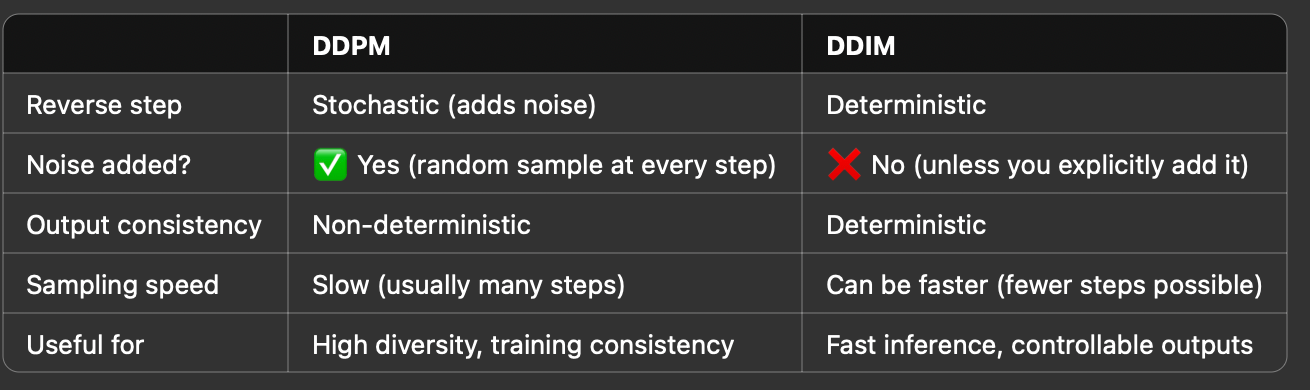
DDPM sampling:

DDIM sampling (deterministic):

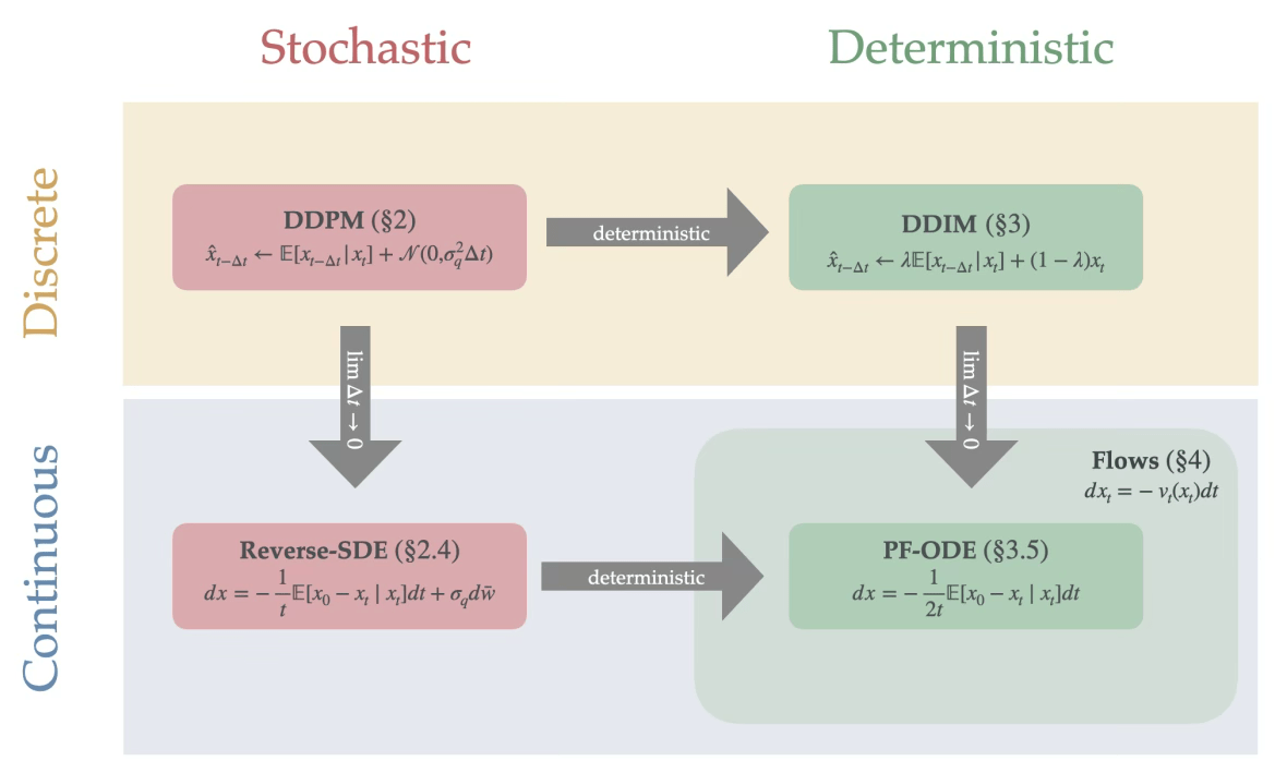
Image credit:  Preetum Nakkiran, “step by step diffusion” https://arxiv.org/pdf/2406.08929

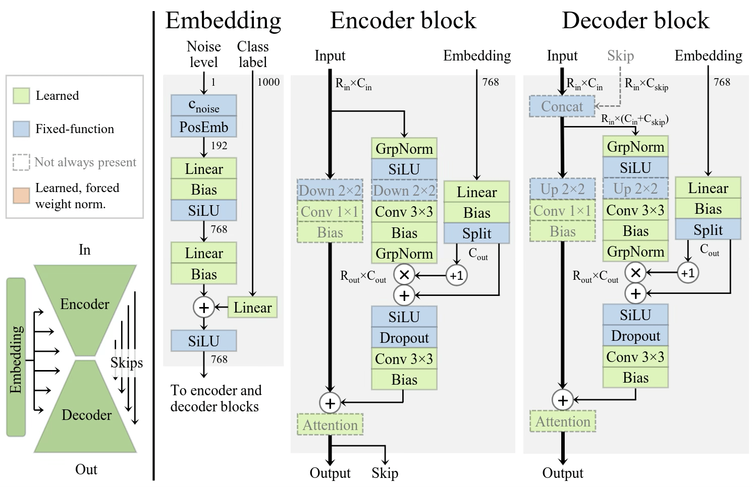
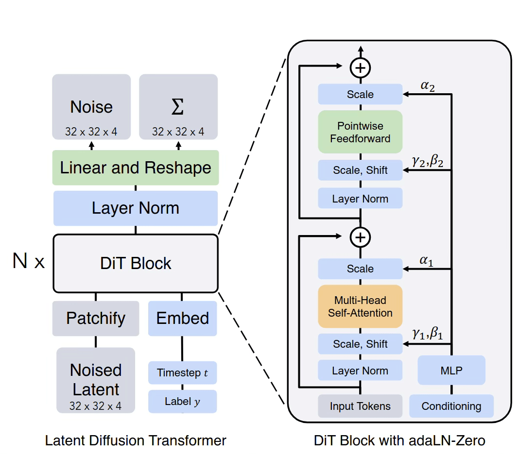
Commonly used architectures

Image credit: (left)Analyzing and Improving the Training Dynamics of Diffusion Models https://arxiv.org/pdf/2312.02696

Right: Scalable Diffusion Models with Transformers https://arxiv.org/pdf/2212.09748

conv U-Net

patch-wise transformers

Just add your conditioning variable \(y\) during training
Works in some cases, usually when the actual \(x\) is low dimensional
Unbiased distribution (in theory)
Doesn’t work in practice when scaled up

Generating \(p(x \mid y)\)

\(p(x \mid y)=\frac{p(y \mid x) \cdot p(x)}{p(y)}\)

Generating \(p(x \mid y)\): Classifier guidance

\(\Longrightarrow \log p(x \mid y)=\log p(y \mid x)+\log p(x)-\log p(y)\)

\(\Longrightarrow \nabla_x \log p(x \mid y)=\nabla_x \log p(y \mid x)+\nabla_x \log p(x)\)

train a classifier on noisy images

\(\Longrightarrow \nabla_x \log p(x \mid y) \approx s\nabla_x \log p(y \mid x)+\nabla_x \log p(x)\)

\(s\)

Image from classifier-free Diffusion Guidance, Ho et.al. 2022

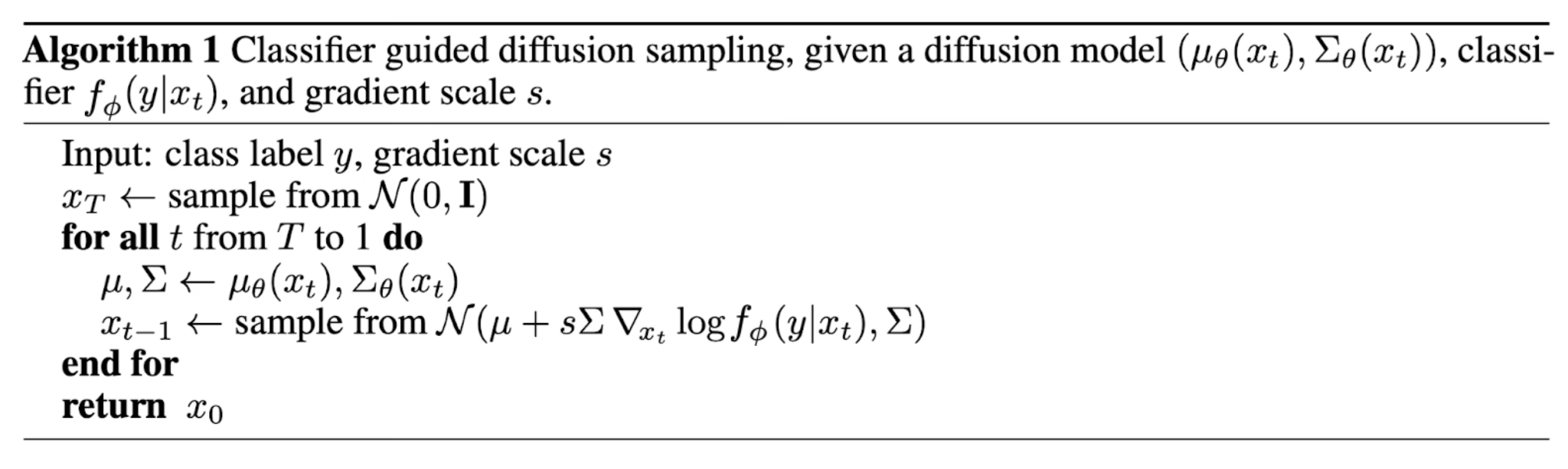
Algorithm from Dhariwal & Nichol, 2021

\( \nabla_x \log p(x \mid y) \approx s\nabla_x \log p(y \mid x)+\nabla_x \log p(x)\)

- Train a classifier on noisy \(x\) (usually undesirable)
- At sampling time, compose its gradient with diffusion score
- Conditional sampling without training a conditional model
- Biased distribution if using a higher guidance strength
- Need discrete classes

Can we generate \(x\) better without training a classifier on noisy \(x\), and also generalize beyond class conditioning like language?

Generating \(p(x \mid y):\)  Classifier guidance

Generating \(p(x \mid y):\)  Classifier-free guidance

\(\nabla_x \log p(x \mid y) \approx s \nabla_x \log p(y \mid x)+\nabla_x \log p(x)\)

\(p(y \mid x)=\frac{p(x \mid y) \cdot p(y)}{p(x)}\)

\(\Longrightarrow \log p(y \mid x)=\log p(x \mid y)+\log p(y)-\log p(x)\)

\(\Longrightarrow \nabla_x \log p(y \mid x)=\nabla_x \log p(x \mid y)-\nabla_x \log p(x)\).

\( \approx s [\nabla_x \log p(x \mid y)-\nabla_x \log p(x)]+\nabla_x \log p(x)\)

• seemingly requires training a conditional diffusion, and an unconditional one
• can share parameter, and train the two together

Control Net

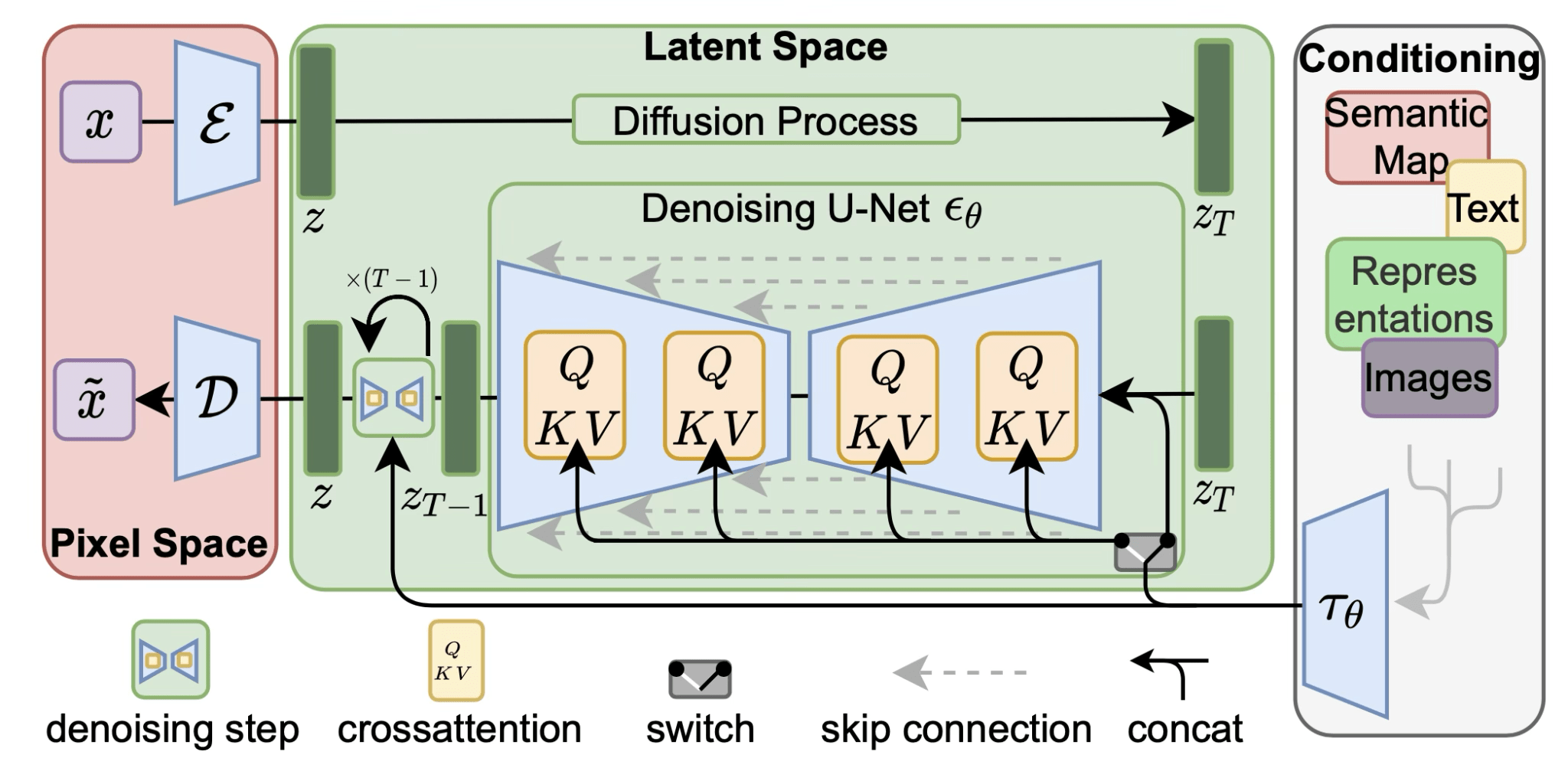
LDM,
Rombach & Blattmann, et al. 2022

U-Net with Conditioning Branch

https://arxiv.org/pdf/2502.09992

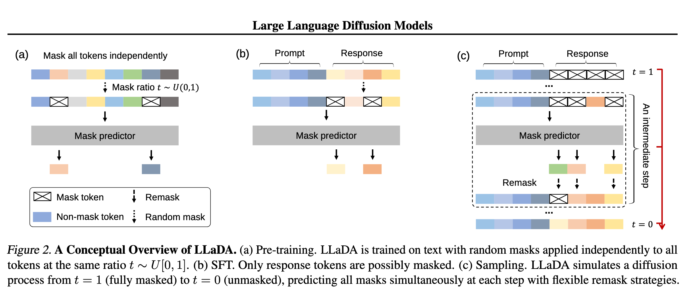
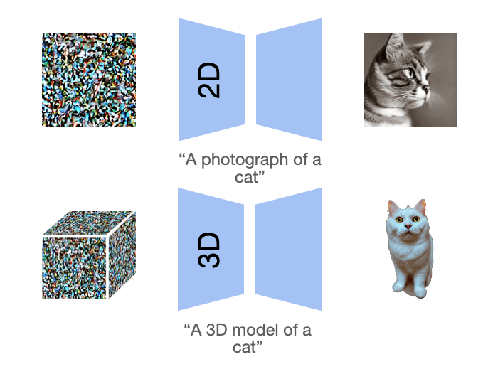
Beyond images?

https://arxiv.org/pdf/2502.09992

Beyond images?

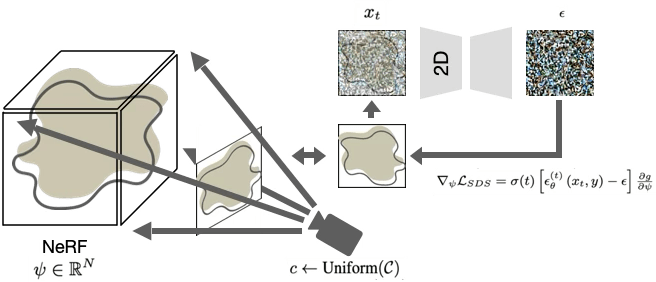
Poole, Ben, et al. "Dreamfusion: Text-to-3d using 2d diffusion." arXiv preprint arXiv:2209.14988 (2022).
Wang, Haochen, et al. "Score jacobian chaining: Lifting pretrained 2d diffusion models for 3d generation." Proceedings of the IEEE/CVF CVPR. 2023.

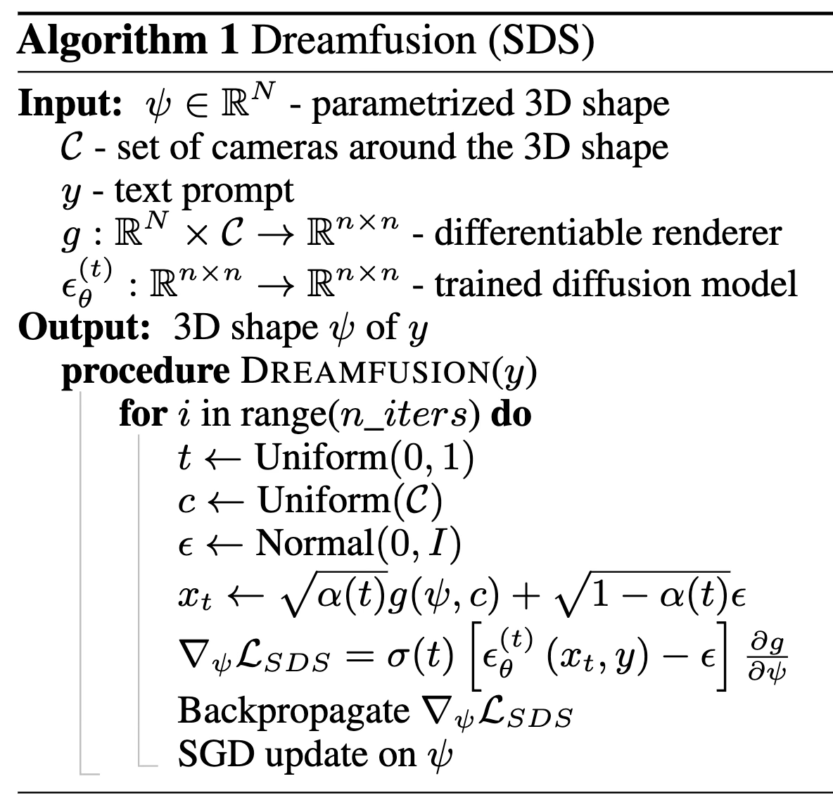
Beyond images?

Poole, Ben, et al. "Dreamfusion: Text-to-3d using 2d diffusion." arXiv preprint arXiv:2209.14988 (2022).
Wang, Haochen, et al. "Score jacobian chaining: Lifting pretrained 2d diffusion models for 3d generation." Proceedings of the IEEE/CVF CVPR. 2023.

Beyond images?

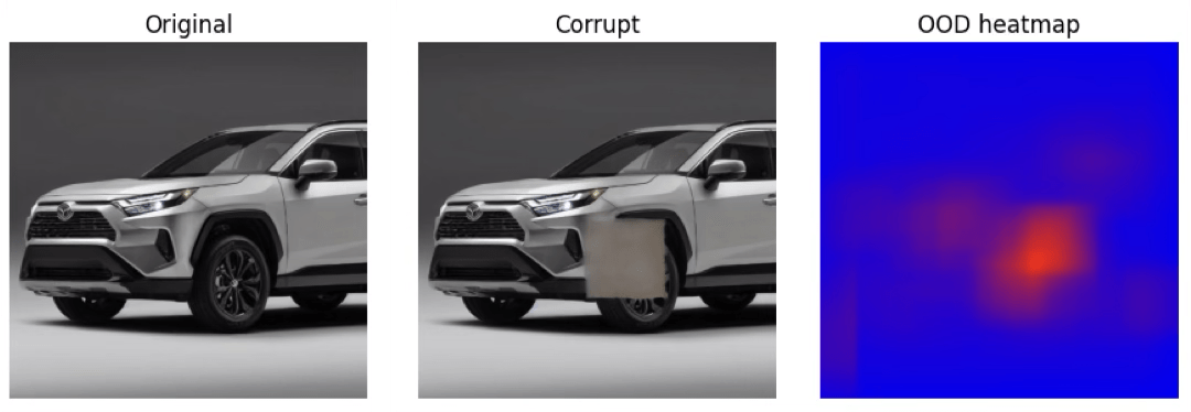
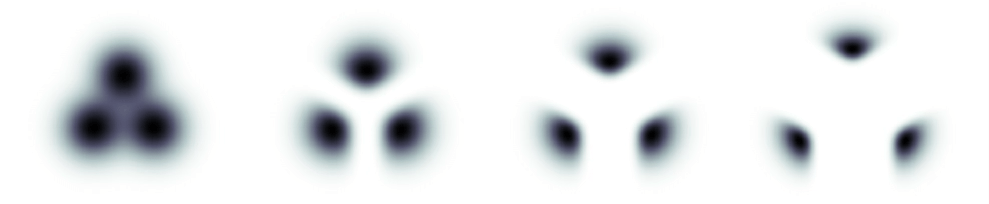
Power law of natural images

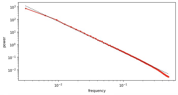
Gaussian noise has uniform power spectral density

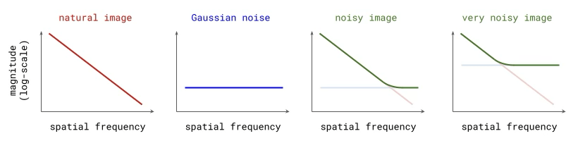
Adding Gaussian noise “drowns out” high frequency features first

for other applications, might worth investigating noise schedule