

Clayton Shonkwiler PRO
Mathematician and artist
TACA 2019
/taca2019
This talk!
Funding: Simons Foundation
Colorado State
Colorado State
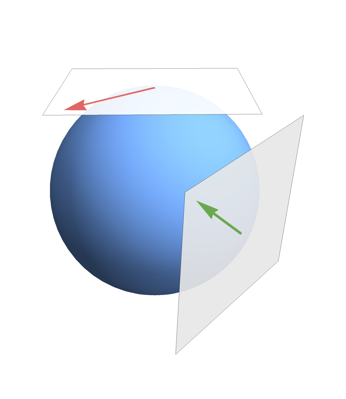
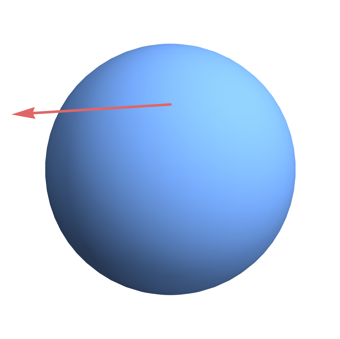
\(M\)
\(T_x M\)
\(x\)
\(y\)
\(u\)
\(v\)
\(T_y M\)
\(u\) and \(v\) live in different vector spaces!
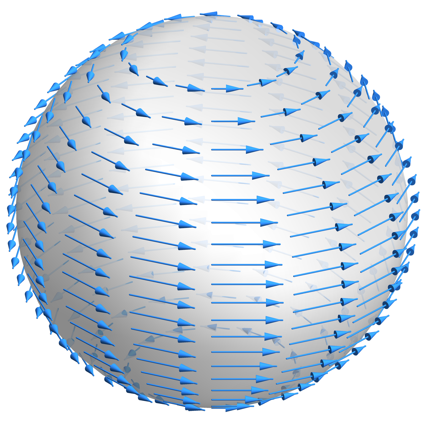
The tangent bundle
A vector field on \(M\) is a (smooth) section of the tangent bundle; i.e., a smooth map \(X: M \to TM\) so that \(\pi \circ X= \operatorname{id}\).
\(\pi\)
Notes:
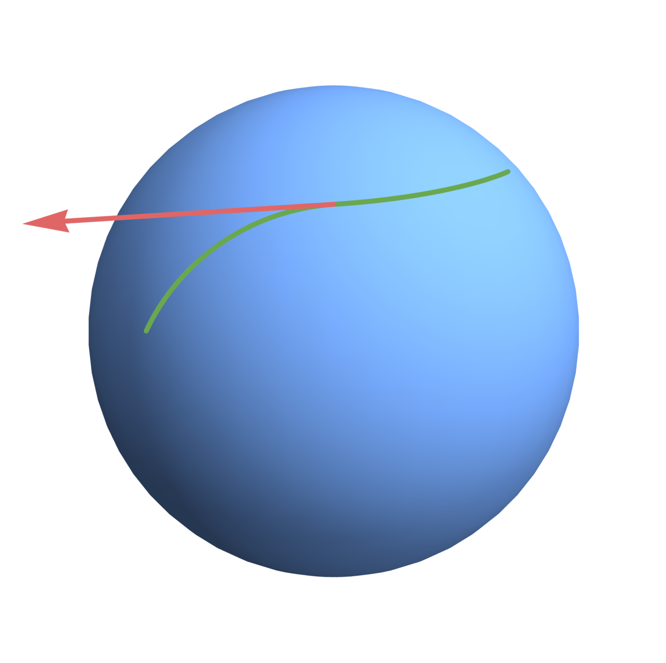
\(M\)
\(x=\gamma(0)\)
\(\gamma'(0)=X(x)\)
\(\gamma(t)\)
\(X \in \mathfrak{X}(M)\) is a differential operator: for \(f \in C^\infty(M)\), \(X(f) \in C^\infty(M)\) is defined by
\(X(x)\)
\(x\)
The Lie bracket \([X,Y](f) := X(Y(f))-Y(X(f))\)
The cotangent bundle
A \(1\)-form on \(M\) is a (smooth) section of the cotangent bundle; i.e., a smooth map \(\omega: M \to T^*M\) so that \(\pi \circ \omega = \operatorname{id}\).
\(\pi\)
Example. If \(f: M \to \mathbb{R}\) is a smooth function, then the differential \(df\) is a 1-form.
The tensor space \(T^p_q(V)\) is the collection of multilinear maps \(\underbrace{V^* \times \dots \times V^*}_p \times \underbrace{V \times \dots \times V}_q \rightarrowtail \mathbb{R}\).
The tensor bundle
\(\pi\)
Implicitly using \(V^{**}\simeq V\): think of \(v \in V\) as a linear functional \(V^* \to \mathbb{R}\) by \(v(\varphi):=\varphi(v)\).
Examples.
(Can also think of \(\mathcal{T}^p_q(M)\) as a tensor product of \(TM\)’s and \(T^*M\)’s over \(C^\infty(M)\).)
The tensor bundle
\(\pi\)
A \((p,q)\)-tensor field (or just \((p,q)\)-tensor) on \(M\) is a (smooth) section of \(\mathcal{T}^p_q(M)\).
Examples. Functions, vector fields, 1-forms.
Example. A Riemannian metric (or metric tensor) is a positive-definite symmetric \((0,2)\)-tensor field \(g\); i.e., \(g(x)=:g_x\) is an inner product on \(T_xM\) for each \(x\).
A Riemannian metric \(g\) on \(M\) is often written as
or just \(g_{ij}\). The notation \(ds^2 = \sum g_{ij}dx^i dx^j = g_{ij}dx^idx^j\) is also common.
Example. \(ds^2=dx^2 + dy^2\) on \(\mathbb{R}^2\) is just the standard dot product:
Example. \(ds^2 = \frac{1}{y^2}\left(dx^2 + dy^2\right)\) on \(\mathbb{H}^2:=\{(x,y) \in \mathbb{R}^2 | y>0\}\) gives the upper half-plane model of the hyperbolic plane.
Definition. Given a smooth curve \(\gamma: [a,b] \to M\), where \((M,g)\) is a Riemannian manifold, then length of \(\gamma\) is
For \(x,y\in M\), the distance from \(x\) to \(y\) is
A differential \(k\)-form on \(M\) is a section of the \(k\)th exterior bundle
\(\pi\)
The space of all \(k\)-forms is denoted \(\Omega^k(M)\).
If \(\omega \in \Omega^k(M)\), then at each \(x \in M\), \(\omega(x)\) is an alternating multilinear map \(T_xM \times \dots \times T_x M \rightarrowtail \mathbb{R}\).
Example. The standard area form on \(\mathbb{R}^2\) is \(dx \wedge dy\).
Example. The standard area form on \(S^2\) is
Think: alternating \((0,k)\)-tensors
The exterior derivative is an anti-derivation \(d\) of degree \(+1\) that makes this a (co)chain complex.
In local coordinates
de Rham’s Theorem. The cohomology of the above cochain complex agrees with the singular cohomology of \(M\) with real coefficients.
Definition. A symplectic form on a manifold \(M\) is a closed, nondegenerate 2-form \(\omega\). The pair \((M,\omega)\) is called a symplectic manifold.
Example. Any area form on an oriented surface; e.g., \((\mathbb{R}^2,dx\wedge dy)\), \((S^2,d\theta\wedge dz)\), \((S^1 \times S^1, ds\wedge dt)\), ...
Example. The canonical form \(\sum dq_i \wedge dp_i\) on \(T^*\mathbb{R}^n\) (or more generally any cotangent bundle).
Darboux’s Theorem. Every symplectic form looks like this locally.
A symplectic manifold must be even-dimensional (over \(\mathbb{R}\)).
\(\omega^{\wedge n} = \omega \wedge \dots \wedge \omega\) is a volume form on \(M\), and induces a measure
called Liouville measure on \(M\).
If \(H: M \to \mathbb{R}\) is smooth, then there exists a unique vector field \(X_H\) (the Hamiltonian vector field for \(H\)) so that \({dH = \iota_{X_H}\omega}\), i.e.,
(\(X_H\) is sometimes called the symplectic gradient of \(H\))
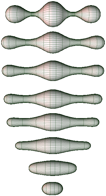
\(H: (S^2, d\theta\wedge dz) \to \mathbb{R}\) given by \(H(\theta,z) = z\).
\(dH = dz = \iota_{\frac{\partial}{\partial \theta}}(d\theta\wedge dz)\), so \(X_H = \frac{\partial}{\partial \theta}\).
Integrating \(X_H\) produces the one-parameter family of diffeomorphisms \(\psi_t(\theta, z) = (\theta+t,z)\).
A (semi-)Riemannian metric \(g\) on \(M\) induces a unique connection called the Levi-Civita connection so that
Christoffel symbols \(\Gamma_{ij}^k\) defined by \(\nabla_{X_i} X_j = \sum_k \Gamma_{ij}^k X_k\)
Definition. An affine connection \(\nabla: \mathfrak{X}(M) \times \mathfrak{X}(M) \to \mathfrak{X}(M)\) satisfies
The Riemann curvature tensor is a \((1,3)\)-tensor field
\(R: \mathfrak{X}(M) \times \mathfrak{X}(M) \to (\mathfrak{X}(M) \to\mathfrak{X}(M))\) defined by
The sectional curvature of a 2-plane \(\sigma \subset T_x M\) is
where \(\{u,v\}\) is any basis for \(\sigma\).
At a point \(x \in M\), the Ricci tensor \(\operatorname{Ric}: T_x M \times T_x M \to \mathbb{R}\) is
Or, in index notation, \(\operatorname{Ric}_{ij} = R_{ikj}^k = g^{k\ell}R_{ki\ell j}\).
For unit \(u \in T_x M\), the Ricci curvature of \(u\) is the value of the corresponding quadratic form: \(\operatorname{Ric}(u,u)\).
Fact. \(\operatorname{Ric}(u,u)\) is \(n-1\) times the average of \(K(\sigma)\) for all 2-planes \(\sigma \subset T_x M\) containing \(u\).
The scalar curvature \(S = \operatorname{tr}_g \operatorname{Ric} = g^{ij}\operatorname{Ric}_{ij}\)
Faraday tensor
(a 2-form)
current 3-form
stress-energy tensor
Einstein tensor: \(G = \operatorname{Ric} - \frac{1}{2} S g\)
Definition. The Grassmannian \(\operatorname{Gr}(d,V)\) is the space of \(d\)-dimensional linear subspaces of the vector space \(V\).
Example. \(\operatorname{Gr}(1,V) =\mathbb{P}(V)\).
Example. \(\operatorname{Gr}(2,\mathbb{R}^4) \simeq (S^2 \times S^2)/(p,q)\sim (-p,-q)\)
\(\{u_1,\dots , u_d\}\) a basis for \(U \subset V\).
With respect to a preferred basis \(\{e_1, \dots , e_n\}\) for \(V\),
Theorem. The image is cut out by a system of quadratic equations (that say the wedge is decomposable).
Example. \(\operatorname{Gr}(2,\mathbb{K}^4)\mapsto\{\Delta_{12}\Delta_{34}-\Delta_{13}\Delta_{24}+\Delta_{14}\Delta_{23}=0\}\)
\(\Delta_U:=d!\, u_1 \wedge \dots \wedge u_d = \sum_{\sigma \in S_d} \operatorname{sgn}(\sigma) u_{\sigma(1)} \otimes \dots \otimes u_{\sigma(d)}\) is an alternating \(d\)-tensor.
where the \(\Delta_{i_1\dots i_d}\) are the determinants of all the \(d \times d\) minors of \([u_1 \cdots u_d]\).
(See Conway–Hardin–Sloane)
Proposition (with Chapman). Let \(V = \mathbb{R}^n\). If \(\Delta_U\) is constructed from an orthonormal basis for \(U\), then
\(\Delta_U(v)\)
\(\operatorname{Proj}_U(v)\)
\(v\)
\(\operatorname{Proj}_U\) is a symmetric \((1,1)\)-tensor.
The flag mean of \(\{U_1,\dots , U_k\} \subset \operatorname{Gr}(d,\mathbb{R}^n)\) is the span of the \(d\) leading (left) singular vectors of \(\operatorname{Proj}_{U_1}+\dots + \operatorname{Proj}_{U_k}\).
Question 1. Is there a notion of tensor SVD so that the flag mean of \(\{U_1,\dots , U_k\}\) is the \(d\) leading (left?) singular vectors of the \(\Delta_{U_1}+\dots+\Delta_{U_k}\)?
Question 2. What is the flag mean of the positive Grassmannian \(\operatorname{Gr}^+(d,\mathbb{R}^n)\), consisting of those \(U\) with all positive Plücker coordinates?
Question 3. Suppose \(U_1,U_2 \in \operatorname{Gr}(d,\mathbb{R}^n)\) and you are given \(a \Delta_{U_1}+b \Delta_{U_2}\) for unknown \(a,b \in \mathbb{R}\). Can you determine \(U_1\) and \(U_2\)?
Question 4. Is there a notion of Grassmannians of tensor subspaces? If so, what are good coordinates on this space?
By Clayton Shonkwiler


