Conditional Formatting

with Formulas

27 slides (22 if you skip the big example at the end)

Click the right arrow to go to the next slide.

Some Basic Rules

1. Make sure you first select the range to format.
2. The range you select should have a rectangular shape. Single cells, rows or columns of any length, and any table-shaped ranges are rectangular.
3. Remember that the formula you write MUST return either TRUE or FALSE. TRUEs get formatted.
4. The formula you write is the test that you want to run for the first cell in the range, i.e., the top left cell of your rectangle.

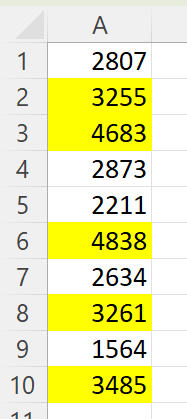
A Simple Example

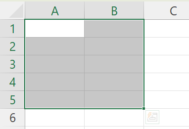
Our range is selected and rectangular.

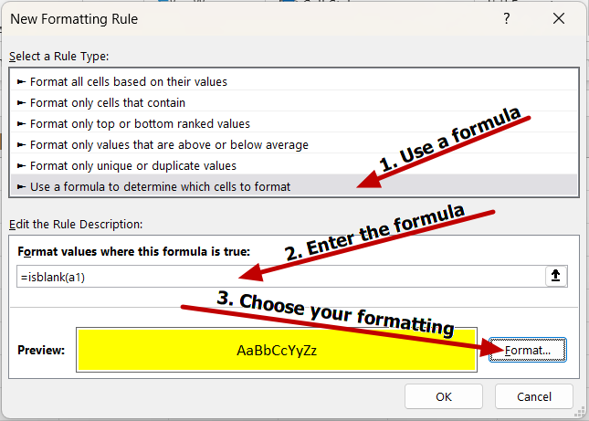
We go to the Home tab of the ribbon and click Conditional Formatting. At the bottom of the menu, select New Rule.

A Simple Example

Our formula will consist only of the ISBLANK function, which returns TRUE if a cell is blank. Our formula should be the test you want to place in the first cell, A1. That test is to see if the cell itself is blank, so it references itself:

=ISBLANK(A1)

Then we set our formatting to highlight yellow.

A Simple Example

A Simple Example

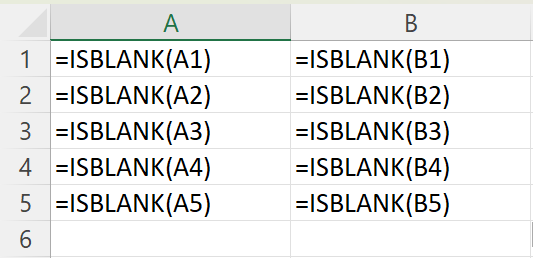
The rule now applies your formula to all cells in the range as if it were copying the formula. So in B1 the formula is =ISBLANK(B1). In A2 it's =ISBLANK(A2) and so forth.

A Simple Example

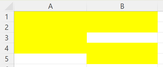
Because I put spaces in cells B3 and A5, they are not blank. So they return FALSE, and, therefore, the rule does not format them.

Fixed Cell References

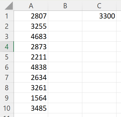
Now let's format cells in a column, A1:A10, that are greater than the value in cell C1.

Fixed Cell References

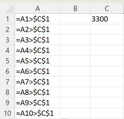
Our formula will be a simple logical test using greater than (>). We'll test the first cell in the range, A1, against the value in cell C1. C1 will have to be a fixed reference so that when the rule "copies" (applies) the formula to each cell, it always compares the cell's value to C1.

=A1>$C$1

Fixed Cell References

Actually, we could have written C$1, but it's a good practice to fully fix cell references when all formulas are referencing the same cell or same range. Here's how the rule is applied.

Fixed Cell References

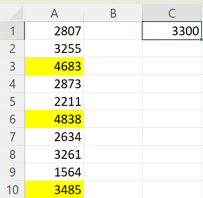
And here's the result.

Fixed Cell References

Likewise, you would use fixed cell references for the range in aggregate functions when used in logical tests like this:

=A1>AVERAGE($A$1:$A$10)

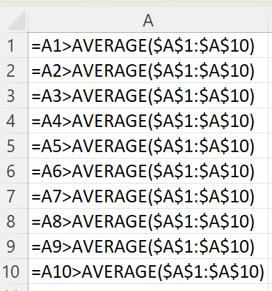
Because all of these AVERAGE functions need the same range

KEY CONCEPT

You write your formula for the first cell.

• The first cell is the top left cell in your selected range.
• The first cell is the first candidate for formatting.
  • Like all cells in the selected range, it gets formatted if its test results in TRUE.
• IMPORTANT: But the test in that cell can apply to ANY cell anywhere in the workbook.
  • Even on another worksheet.

Test One Cell, Highlight Another

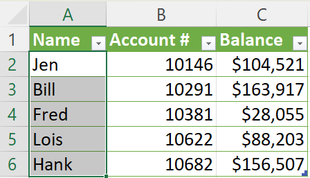
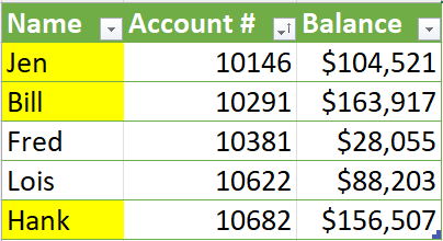
For example, let's say you want to highlight the name of anyone in this table who has more than $100,000 in their account. 

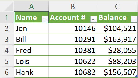
So we test the Balance column but apply the formatting to the Name column. Begin by selecting the Name column.

Test One Cell, Highlight Another

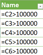
The first cell is A2. That's the first candidate for formatting. But the formula for A2 will not have a reference to A2. Instead it will need to reference (test) C2 to see if it's greater than $100,000.

So the formula for the first cell, A2, is:

=C2>100000

Test One Cell, Highlight Another

So we select A2:A6 to identify the candidate cells for formatting. Then apply our formula to those cells.

Test One Cell, Highlight Another

The rest of this slide set is an example.

If you're not interested in how to highlight protected and unprotected cells, you can skip to the recap.

Message from the Inspector General

Advantage of Formulas

Obviously, there are easier ways to conditionally format cells without writing formulas. But sometimes you need something for which there is no preset or new rule type.

For example, what if I had spent hours unlocking individual cells in multiple worksheets in a workbook, so that I could protect (lock) the worksheets and prevent users from editing the wrong cells.

But I've lost track of which cells are locked and want to quickly find them. This is a pretty obscure problem for which there is no preset or regular new-rule functionality.

Advantage of Formulas

No worries. We can use a formula, specifically the CELL function.

The CELL function can check the cell's many properties for matches and return a TRUE or FALSE outcome. (Go here for a list of those properties.)

For our situation, we're checking to see if the cell has the "protect" property set. This means the cell is locked.

Advantage of Formulas

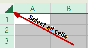
We'll start with selecting an entire worksheet by clicking the triangle above and to the left (northwest) of cell A1.

Then go make a new rule with a formula and type the following:

=CELL("protect", A1)

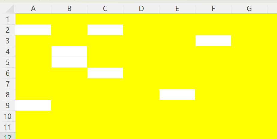
Select your formatting (I'll use yellow highlighting again) and apply the rule to every cell in the worksheet.

Advantage of Formulas

The rule highlights all the cells that are locked.

Advantage of Formulas

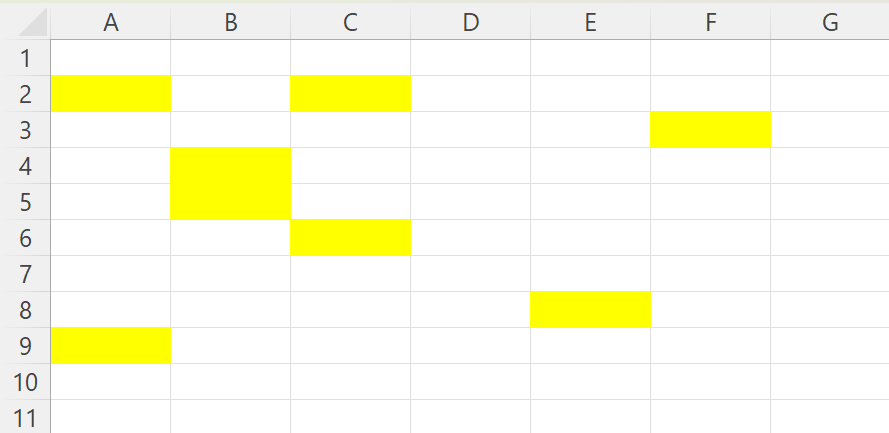
It'd be better to highlight the cells that aren't locked. To do that, nest the CELL function inside a NOT function*.

=NOT(CELL("protect", A1))

* The NOT function turns TRUEs into FALSEs and FALSEs into TRUEs.

Recap

• Select your range to format before choosing Conditional Formatting. Make your selection rectangular. (Yes, it's possible for it not to be.)
• Write your formula so that it results in a Boolean value, i.e., either TRUE or FALSE.
• Write the formula so that it formats the first cell in your selected range if TRUE. That's the top left cell of your rectangle.
• Be sure to use dollar signs ($) for fixed cell references.

One Final Tip

You can pretest your formula's effect on each cell in the range by typing out and copying the formula across a blank area the size of your range. Or just test part of it.

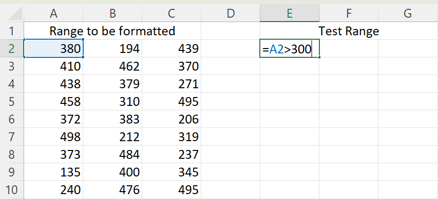
your formula

Copy here

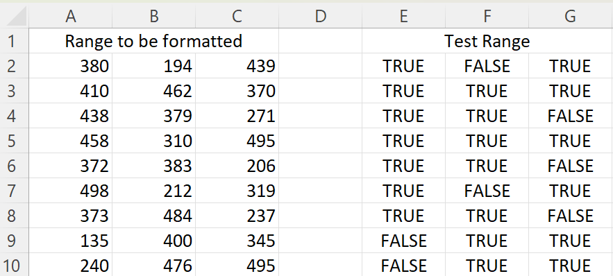
One Final Tip

This shows you which cells will test TRUE and which test FALSE. Did the formula find all cells >300? Looks like it.

A big muy appreciado to Microsoft MVP and Excel genius/beast Mike Girvin for this tip. Check him out at ExcelisFun.

Fin