Data Structure Deep Dive
Recap
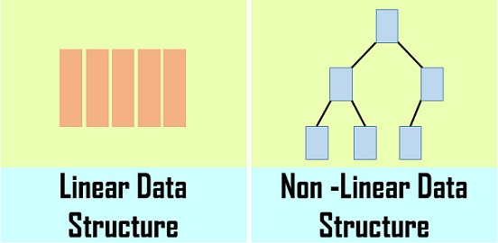
Linear Data Structures: A linear data structure traverses the data elements sequentially, in which only one data element can directly be reached.
Non-Linear Data Structures:
Every data item is attached to several other data items in a way that is specific for reflecting relationships. The data items are not arranged in a sequential structure.
Objectives
- Complexity
- Array
Complexity
- A way of comparing how different algorithms perform in an objective manner that doesn’t rely on hardware.
- We look at the number of steps that it takes to execute an algorithm and we call this the time complexity.
- Time Complexity : the number of steps involved to run an algorithm.
- Memory Complexity : the amount of memory it takes to run an algorithm.
Big-O Notation
- Big O notation is used in Computer Science to describe the performance or complexity of an algorithm.
- Big O specifically describes the worst-case scenario and the execution time required or the space used by an algorithm.
The use of Big O
It can measure how the performance of an algorithm changes, based on the size of the input set of data.
The reason the letter O (in Big-O) is used is because the growth rate of an algorithm’s time complexity is also referred to as the order of operation.
It usually describes the worst case scenario of how long it takes to perform a given operation. And it’s important to note that many different algorithms and data structures have more than one Big-O value.
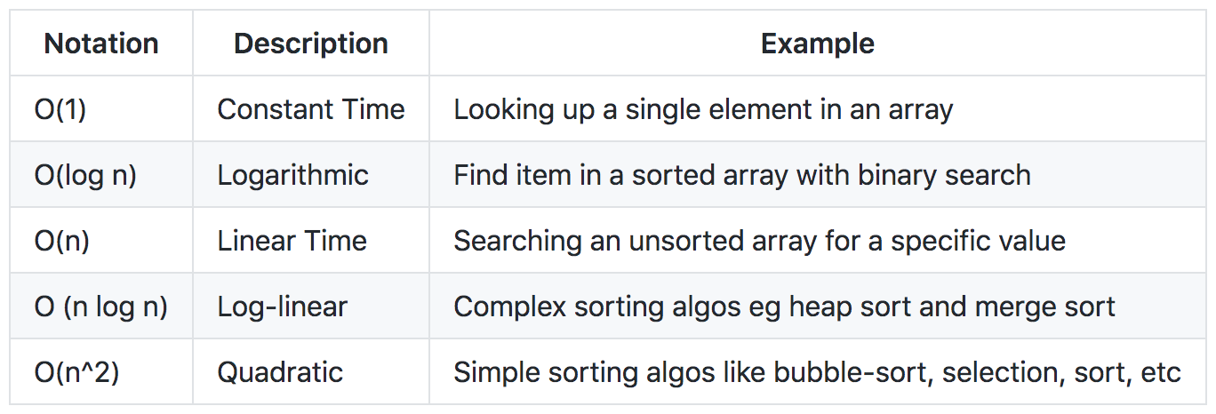
Examples of Big O notations
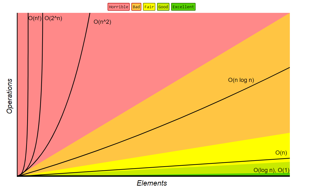
-
O(1) (best case): Given the page that a business's name is on and the business name, find the phone number.
-
O(1) (average case): Given the page that a person's name is on and their name, find the phone number.
-
O(log n): Given a person's name, find the phone number by picking a random point about halfway through the part of the book you haven't searched yet, then checking to see whether the person's name is at that point. Then repeat the process about halfway through the part of the book where the person's name lies.
The phone book as an example to compare other kinds of operations and their running time.
-
O(n): Find all people whose phone numbers contain the digit "5".
-
O(n log n): There was a mix-up at the printer's office, and our phone book had all its pages inserted in a random order. Fix the ordering so that it's correct by looking at the first name on each page and then putting that page in the appropriate spot in a new, empty phone book.
How to Determine Complexities
- Sequence of statements: If each statement is "simple" then the time for each statement is constant and the total time is also constant: O(1)
- if-then-else statements: if sequence 1 is O(N) and sequence 2 is O(1) the worst-case time for the whole if-then-else statement would be O(N).
- for loops: The loop executes N times, so the sequence of statements also executes N times. Since we assume the statements are O(1), the total time for the for loop is N * O(1), which is O(N) overall.
- Nested loops: the total complexity for the two loops is O(N^2).
Array
- Homogeneity: all elements are of the same data type, hence homogeneous data

- Array elements are stored at contiguous memory locations

Arrays in Memory
- Contiguouts block in memory.
- Every element occupies the same amount of space in memory.
- If an array starts at memory address x, and the size of each element in the array is y, we can calculate the memory address of the ith element by using the following expression: x + i * y.
- If we know the index of an element, the time to retrieve the element will be the same, no matter where it is in the array.
- They’re also memory efficient because we don’t have to store any extra information with each element in the array.
Type of Array
- One dimensional (just a linear list): only one subscript is required to access an individual element
2. Two dimensional (matrix/table): two indices/subscripts are required (row, column)


Search for a target (key) in the search space Search space examples are:
- All students in the class
- All numbers in a given list
One of the two possible outcomes
Target is found (success)
Target is not found (failure)
Searching Algorithms
Search in a sequential order
Termination condition
- Target is found (success)
- List of elements is exhausted (failure)
Sequential Search
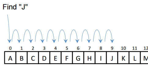
Given: A list of N elements, and the target
1. index <-- 0
2. Repeat steps 3 to 5
3. Compare target with list[index]
4. if target = list[index] then
return index // success
else if index >= N - 1
return -1 // failure
5. index <-- index + 1
Sequential Search Algorithm
Complexity: O(n): it contains single loop
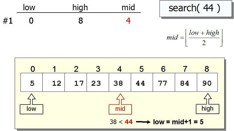
Binary Search
Search through a sorted list of items
Sorted list is a pre-condition for Binary Search!
Repeatedly divides the search space (list) into two
Divide-and-conquer approach
1. Divide: Break the given problem into subproblems of same type.
2. Conquer: Recursively solve these subproblems
3. Combine: Appropriately combine the answers
Binary Search Algorithm
Middle <- (LI + HI) / 2
One of the three possibilities
Key is equal to List[Middle]
o success and stop
Key is less than List[Middle]
o Key should be in the left half of List, or it does not exist
Key is greater than List[Middle]
o Key should be in the right half of List, or it does not exist
Termination Condition
List[Middle] is equal to Key (success) OR LI > HI (Failure)
Complexity: O(log n)
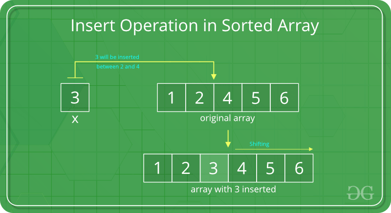
Insertion Algorithm
Insert operation is to insert one or more data elements into an array. Based on the requirement, a new element can be added at the beginning, end, or any given index of array.
Deletion Operation
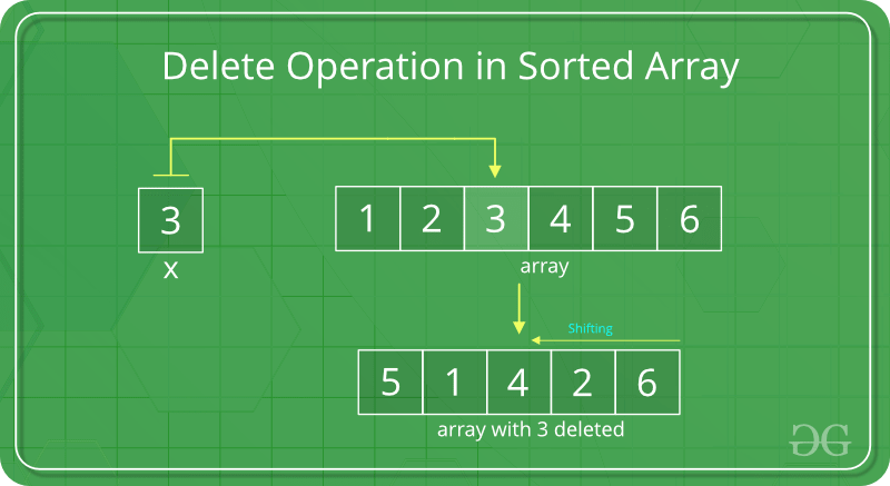
In delete operation, the element to be deleted is searched using binary search and then delete operation is performed followed by shifting the elements.
Sort Algorithm
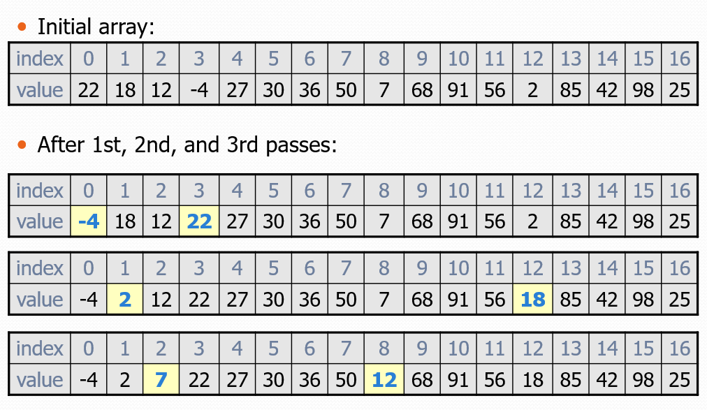
Selection sort: Orders a list of values by repeatedly putting the smallest or largest unplaced value into its final position.
The algorithm:
Look through the list to find the smallest value.
Swap it so that it is at index 0.
Look through the list to find the second-smallest value.
Swap it so that it is at index 1.
Repeat until all values are in their proper places.
Sort Algorithm
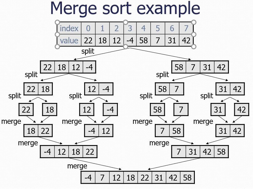
Merge sort: Repeatedly divides the data in half, sorts each half, and combines the sorted halves into a sorted whole.
The algorithm:
Divide the list into two roughly equal halves.
Sort the left half.
Sort the right half.
Merge the two sorted halves into one sorted list.
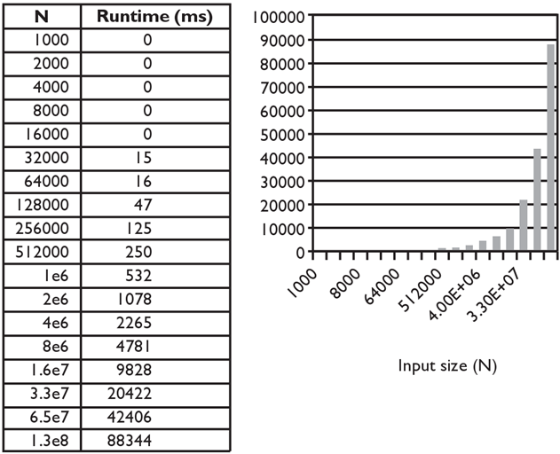
Merge sort runtime
- Bubble sort is a simple sorting algorithm. This sorting algorithm is comparison-based algorithm in which each pair of adjacent elements is compared and the elements are swapped if they are not in order.
- This algorithm is not suitable for large data sets as its average and worst case complexity are of Ο(n^2) where n is the number of items.
Sort Algorithm
Bubble Sort Algorithm
Initialize the size of the list to be sorted to be the actual size of the list.
Loop through the list until no element needs to be exchanged with another to reach its correct position.
Loop (i) from 0 to size of the list to be sorted - 2.
Compare the ith and (i + 1)st elements in the unsorted list.
Swap the ith and (i + 1)st elements if not in order ( ascending or descending as desired).
Decrease the size of the list to be sorted by 1.

2) Bubble sort starts with very first two elements, comparing them to check which one is greater.

1) We take an unsorted array for our example. Bubble sort takes Ο(n^2) time so we're keeping it short and precise.
3) Next, we compare 33 with 27. we find that 27 is smaller than 33 and these two values must be swapped.

5) We know then that 10 is smaller 35. Hence they are not sorted then swap
4) Next we compare 33 and 35. We find that both are in already sorted positions.
6) We swap these values. We find that we have reached the end of the array. Repeat the same step until it is fully sorted


Indexing: inspect or update an element using its index. Performance is very fast O(1)
randomNumber = numbers[5];
numbers[20000] = 100;
Insertion: add an element at certain index
– Start: very slow O(n) because of shift
– End : very fast O(1) because no need to shift
Removal: remove an element at certain index
– Start: very slow O(n) because of shift
– End : very fast O(1) because no need to shift
Array Operations and Big O notatitons
Array Operations and Big O notatitons
Search: performance depends on algorithm
1) Linear: slow O(n)
2) Binary : O(log n)
Sort: performance depends on algorithm
1) Bubble: slow O(n2)
2) Selection: slow O(n2)
3) Merge : O(n log n)
Thank you
Data Structure Deep Dive
By Sofwan Abdulwahab
Data Structure Deep Dive
- 588


