MTD 350
Mini Project Mid-Semester Presentation

Kartikay Garg - 2013MT60600
Somanshu Dhingra - 2013MT60622
Supervisor:
Prof. Nilhadri Chatterjee
Aim:
Parallelised implementation of various Machine Learning techniques on Apache Spark using the MapReduce paradigm.
-
Get familiar with MapReduce paradigm and programming frameworks based on it esp. Apache Spark.
-
Learn parallelisation of Machine Learning Algorithms
-
Explore new algorithms to be implemented using MapReduce.
-
Simulate these algorithms on large data-sets to observe & compare their performance meanwhile generating useful results on them.
MapReduce:
Programming paradigm for implementing parallel & distributed algorithms on clusters.
MAP : Each node takes its local records as input and creates a key/value pair as output.
SHUFFLE : All the key/value pairs are sorted and redistributed such that all pairs having same key belongs to same node.
REDUCE : Each set of these pairs is reduced in parallel to again give a single key/value pair which forms the output.
Machine Learning Algorithms in MapReduce:
Most of the machine learning algorithms evaluates some function usually in summation form over the entire data.
Thus, for all these algorithms the calculations can be easily distributed over multiple cores to achieve linear speedup.
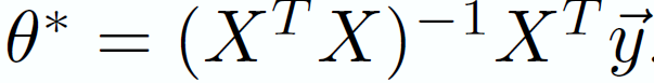
For Example, in ordinary linear regression the optimal coefficients are found using the formula,
The matrix multiplication can be written in summation form and be distributed over multiple nodes
Many popular machine learning techniques have been written and implemented in MapReduce form as available in the Mlib Library of Apache Spark
Apache Spark:
k-Nearest Neighbor (kNN)
Given a set P of points in d-dimensional space, the aim is to construct a data structure that given a query point q, finds its nearest neighbor in P.
It has extensive application in learning of feature-rich data and computational data.
Challenge:
As the number of dimensions increase, the space and time complexity may increase exponentially.
Roughly, time complexity ~
and, space complexity ~
O(n^{O(d)})
O(d^{O(1)}logn)
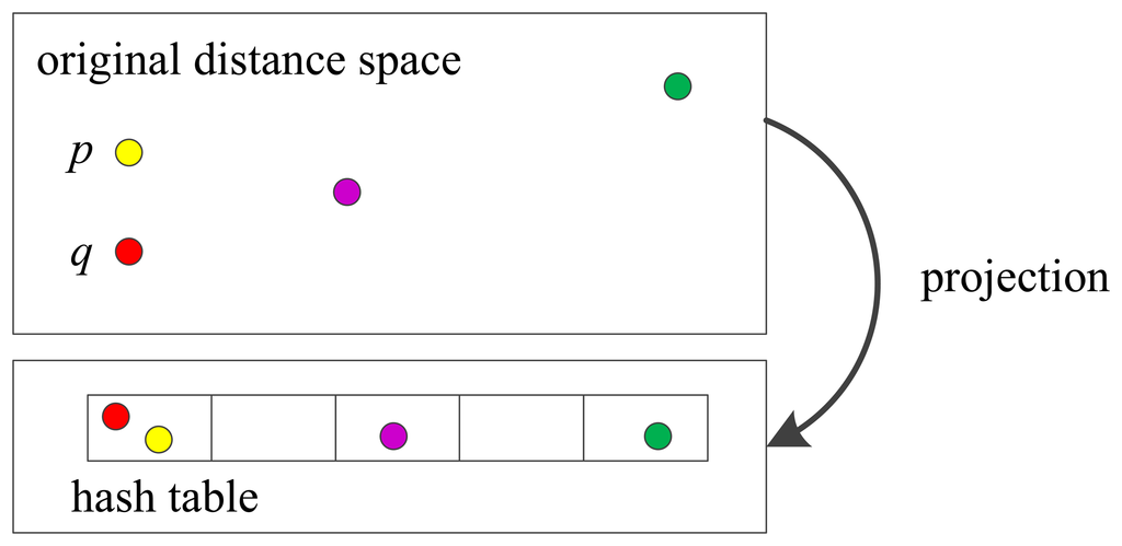
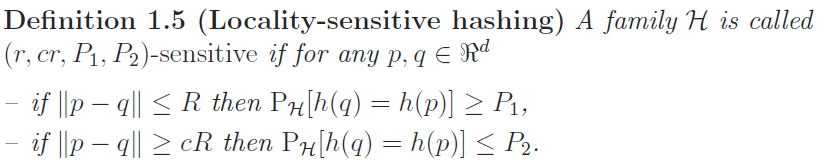
Locality Sensitive Hashing (LSH)
It is the most extensively practically used approach.
Its main idea is to hash the data points using several hash functions so as to ensure that, for each function, the probability of collision is much higher for points which are close to each other than for those which are far apart. Then, one can determine near neighbors by hashing the query point and retrieving elements stored in buckets containing that point.
LSH (contd.):
Construct L number of k-dimension hash functions:
where
is independently and uniformly chosen at random from H
Thus, this family of hash functions G is a
sensitive family and hence more reliable.
h_{t,j} (1\leq t \leq k, 1 \leq j \leq L)
g_{j}(q) = (h_{1,j}(q), h_{1,j}(q), . . . , h_{k,j}(q))
(r,cr,P_{1}^{k},P_{2}^{k})
h_{a,b}(\vec{v}) = \lfloor \frac{\vec{a}.\vec{v} + b}{W} \rfloor
An easy and efficient choice for hash function family, H is :
where, a is vector in d-dimension space chosen uniformly from a p-stable distribution,
W is the size of each bucket
and b is a random value chosen uniformly from [0,W]
h_{a,b} : \mathbb{R}^{d} \mapsto \mathbb{Z}
Using the above we now create a set ,G of hash functions of cardinality L and each hash function a k-tuple of different hash functions picked randomly from H.
LSH (contd.):
LSH-based KNN using MapReduce:
Complexity Analysis:
The algorithm helps in achieving linear speed up both in the pre-processing and query time.
Given : p number of nodes in the cluster,
n number of data points,
d dimension of the space
L number of hashing functions in G each having k functions concatenated from H
Pre-processing time ~
Query TIme ~
Space Complexity ~
\theta ^{*} = (X^{T}X)^{-1} (X^{T} \vec{y})
\theta ^{*} = A^{-1}B
A = (X^{T}X) = \sum_{i=1}^{m} (x_{i}x_{i}^{T})
B = X^{T} \vec{y} = \sum_{i=1}^{m}x_{i}y{i}
Map
\sum_{subgroup} (x_{i}x_{i}^{T})
Reduce
A
\sum_{subgroup}x_{i}y{i}
B
Linear Regression
MTD 350
By Somanshu Dhingra


