

Stefan Sommer
Professor at Department of Computer Science, University of Copenhagen
Faculty of Science, University of Copenhagen
Stefan Sommer
Department of Computer Science, University of Copenhagen
\( \phi \)
Session 1: (L 9-9:45) Shape analysis and actions of the diffeomorphism group
Session 2: (E 10-10:45) Landmark analysis in Theano Geometry
Session 3: (L 11-11:45) Linear representations and random orbit model
Session 4: (E 12:30-13:15) Landmarks statistics in Theano Geometry
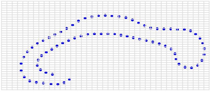
Session 5: (L 13:30-14:15) Shape spaces of images, curves and surfaces
Session 6: (E 14:30-15:15) Analysis of continuous shapes
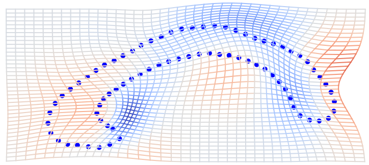
\( \phi\in\mathrm{Diff}(\Omega) \) diffeomorphism of domain \(\Omega\)
\( \phi \)
Variational problem to find optimal \(\phi\in G\):
\( \phi_t:[0,T]\to\mathrm{Diff}(\Omega) \) path of diffeomorphisms (parameter t)
Constructing diffeomorphisms:
Forward flow:
\[ \frac{d}{dt}\phi(x,t)= v(\phi(x,t),t) ,\ \forall x\in\Omega \]
\(\phi(x,0)=x\)
\(\phi_t\in G=\mathrm{Diff}(\Omega)\)
\(v_t\) is a vector field on \(\Omega\): \(v\in V\subset \mathcal{X}\)
It is the Eulerian velocity that controls the flow
The family \(v_t\), \(t\in [0,T]\) determines the flow
Variational problem:
\( E_{s_0,s_1}(\phi)=\mathrm{min}_{\phi_t}R(\phi_t)+\frac1\lambda S(\phi_T.s_0,s_1) \)
\(R(\phi_t):=\int_0^T\|\partial_t \phi_t\|_{\phi_t}^2dt\), \(v_t=\partial_t\phi_t\circ\phi_t^{-1}\)
So we need a norm on \(V\) for defining \(\|\partial_t\phi_t\|_{\phi_t}=\|v_t\|\)
Norm on \(V\) is defined via a Reproducible Kernel Hilbert Space (RKHS) structure
Velocity \(v\)
Momentum \(m=Lv\) (recall: \(p\) for landmarks)
\(L\) is the momentum operator \(L:V\to V^*\)
Kernel \(K\) is the inverse momentum: \(K=L^{-1}\)
\(K\) is as well a matrix-valued function on \(\Omega\times\Omega\): \[K: \Omega\times\Omega\to\mathbb{R}^{d\times d}\]
e.g. \(K(x,y)=\alpha e^{-\frac{\|x-y\|^2}{2\sigma^2}}\)
Kernel \(K\) is the inverse momentum: \(K=L^{-1}\)
\(K\) is as well a matrix-valued function on \(\Omega\times\Omega\): \[K: \Omega\times\Omega\to\mathbb{R}^{d\times d}\]
e.g. \(K(x,y)=\alpha e^{-\frac{\|x-y\|^2}{2\sigma^2}}\)
For \(a\in\mathbb{R}^d\), \(K(\cdot,x)a\in V\)
\[\langle K(\cdot,x)a,K(\cdot,y)b \rangle= a^TK(x,y)b \]
\(V\) is the completion of finite linear combination of \(K(\cdot,x)a\)
\(V\) is embedded in \(L^2(\Omega,\mathbb{R}^d)\)
\(V\) is the completion of finite linear combination of \(K(\cdot,x)a\)
\(V\) is embedded in \(L^2(\Omega,\mathbb{R}^d)\)
vector \(w\in L^2(\Omega,\mathbb{R}^d)\) gives covector
\(v\mapsto\int_\Omega w(x)^Tv(x)dx\)
velocity vectors \(v_t\) are often smooth
momenta \(m_t=Lv_t\) are often rough
e.g. Dirac deltas:
\(v_t=\sum_{i=1}^NK(\cdot,x_i)a_i\)
\(m_t=\sum_{i=1}^Na_i\otimes\delta_{x_i}(\cdot)\) i.e. landmark momenta \(p_i=a_i\otimes\delta_{x_i}(\cdot)\)
The norm \(\|\partial_t\phi_t\|_{\phi_t}^2\) determines a Riemannian metric (that's why we draw \(G\) curved)
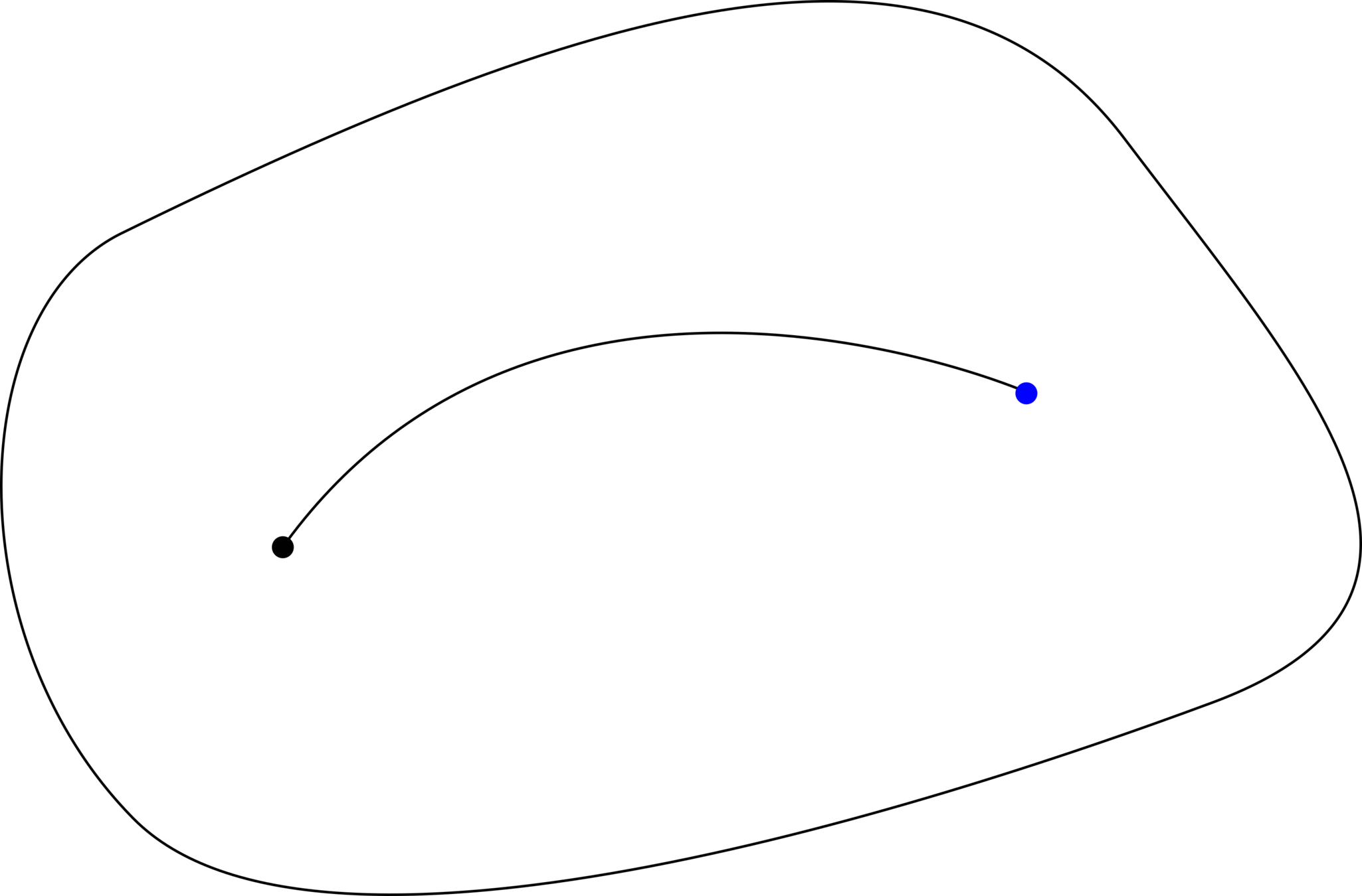
Riemannian geodesics, length/energy minimizing:
\[\phi_t=\mathrm{argmin}_{\phi_t}\int_0^T\|\partial_t\phi_t\|_{\phi_t}^2dt\]
\(v_0=\partial_t\phi_t|_{t=0}\) determines evolution
\(\mathrm{Exp}:V\to G\) endpoint map
\(\mathrm{Log}:G\to V\) initial velocity map
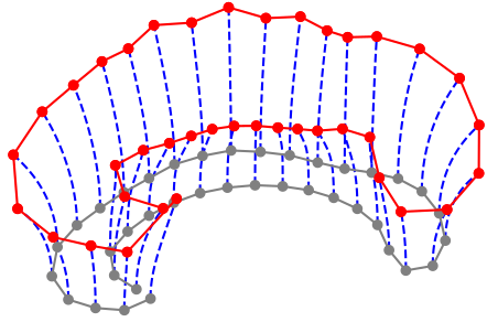
\(\pi\) is a Riemannian submersion
it induces a Riemannian metric on \(\mathcal{S}\)
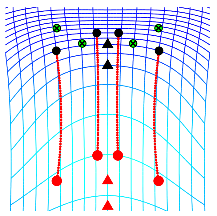
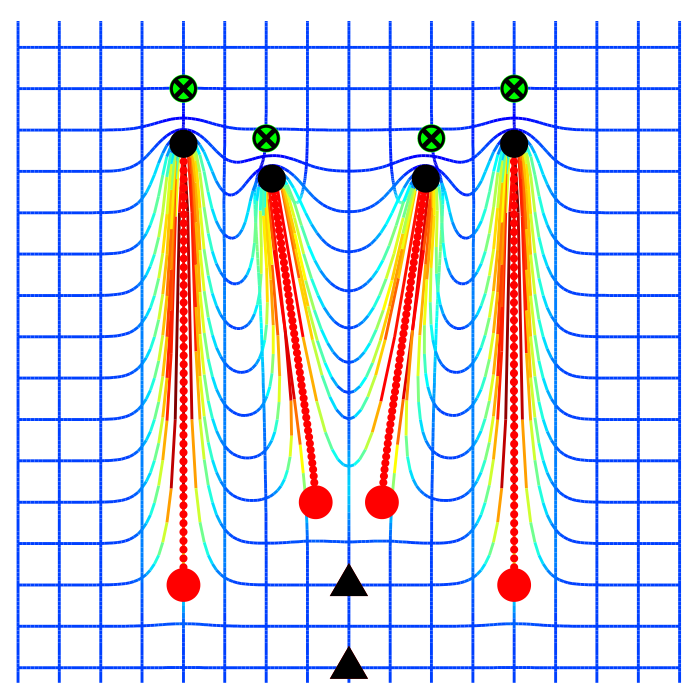
Geodesics on \(\mathcal{S}\) lift to
horizontal geodesics on \(G\)
Horizontal geodesics on \(G\)
project to geodesics on \(\mathcal{S}\)
Those were the landmark geodesics
But we can do this for any shape space
Exp/Log maps are defined on \(\mathcal{S}\) as well
\(V\) is a vector space (infinite dimensional)
We can perform regular statistics on \(V\)
Normal distribution \(N(0,\Sigma)\) maps to distribution \(\mathrm{Exp}_*N(0,\Sigma)\) on \(G\) - random orbits
Data \(s_1,\ldots,s_N\) can be analysed
in \(V\): \(v_i=\mathrm{Log}(s_i)\)
Template estimation (mean shape/image):
\[s_0=\mathrm{argmin}_{s\in\mathcal{S}}\sum_{i=1}^nd(s,s_i)^2\]
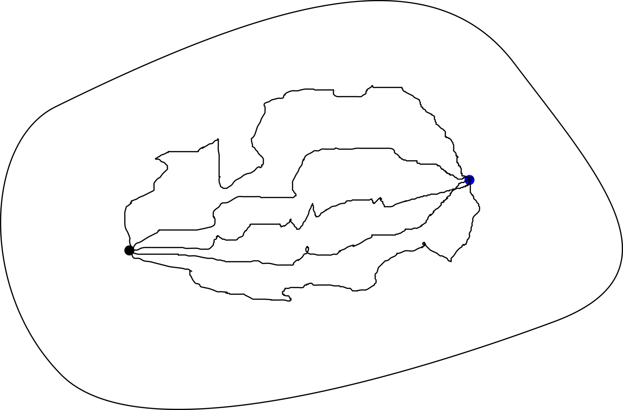
Geodesic distance on \(\mathcal{S}\):
\[d(s,s_i)=\argmin_{\phi_t,\phi_T.s=s_i}\int_0^T\|v_t\|^2dt\]
Tangent space Principal Component Analysis:
\[\mathrm{PCA}(\mathrm{Log}(s_0,s_1),\ldots,\mathrm{Log}(s_0,s_n))\]
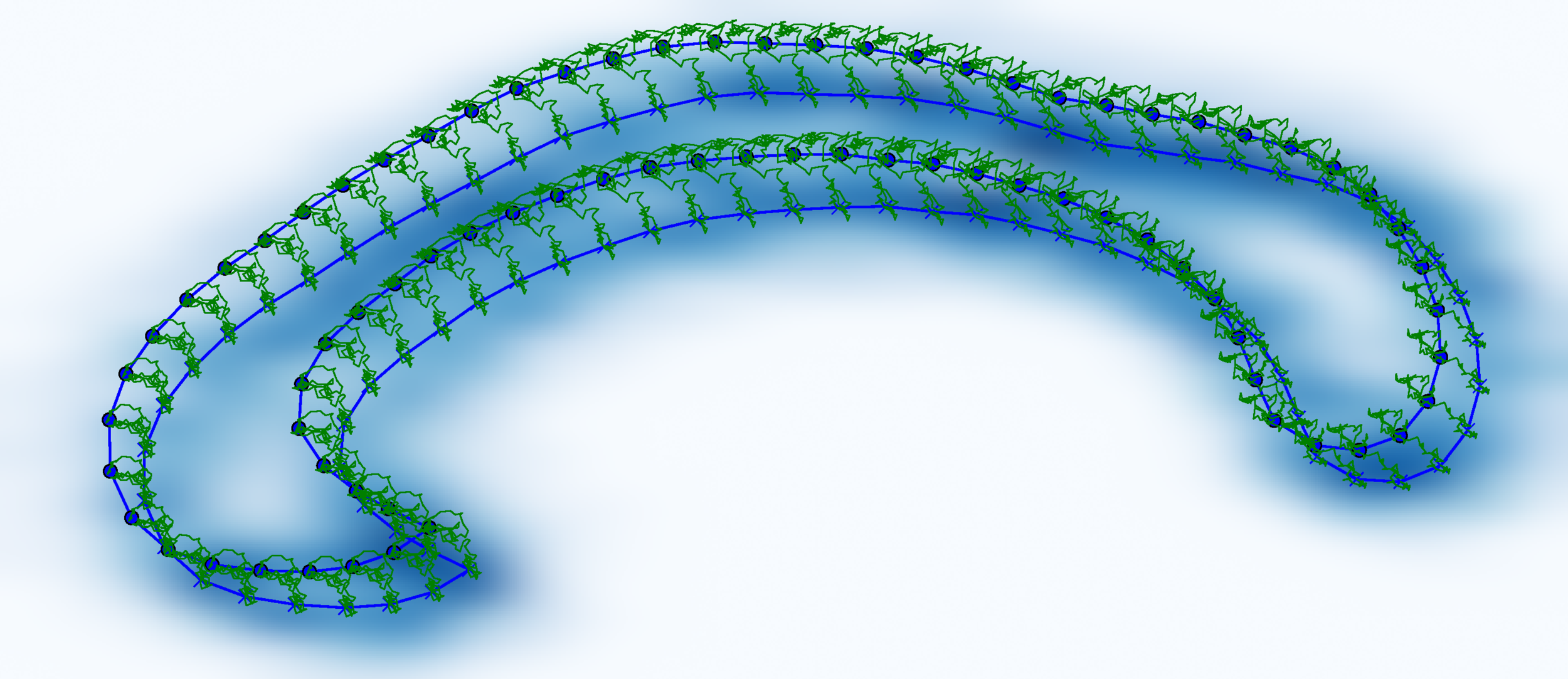
e.g. Riemannian Brownian motion
Exercise session:
hint: use a low number of landmarks to reduce computation time
By Stefan Sommer


