Quantum Fourier Transform and Applications

Agenda
-
Motivation
-
Basics of Quantum Computing
-
Overview of Fourier Transform
-
Quantum Fourier Transform
-
Applications
Motivation
Fourier Transform Applications
Used to decompose a signal into its constituent frequencies. Employed heavily in signal processing, and almost all of our electronics rely on it.
The discrete Fourier transform can sample an unknown periodic function to find its period. This is called period finding and has a wide range of applications, including factoring of numbers into primes.
Fast Fourier Transform
Used to compute the discrete Fourier transform of a sequence of samples.
Widely considered one of the most important numerical algorithms ever developed.
Reduces complexity of computing DFT from \(O(n^2)\) to \(O(nlogn)\) where \(n\) is the data size. Uses a divide and conquer strategy.
However, there are cases where FFT is not efficient enough, like in analyzing MRI data (where approximations must be used), or in period finding (like factoring into prime numbers).
Quantum Fourier Transform
Computes the discrete Fourier transform with an exponential speedup over FFT!
Computes DFT of \(2^n\) elements in \(O(n^2)\) time where FFT would take \(O(n2^n)\) time.
This speedup allows for efficient algorithms for factoring, discrete logarithm, and the hidden abelian subgroup problem.
But there's a catch
Limitations of QFT
Because the \(2^n\) numbers are stored in \(n\) an n qubit register, we can compute the QFT of all of those numbers, but can only extract \(n\) pieces of data at a time.
However, in many cases this is not a problem since we are interested in the expected value of an operator over the \(2^n\) Fourier coefficients. This is the case in period finding where we can extract the period \(r\) by applying an operator to the Fourier coefficients.
Basics of Quantum Computing
Qubits
The fundamental unit of quantum computing is the qubit - often but not necessarily implemented using electrons.
Electrons have a property called spin, which behaves like angular momentum and induces a magnetic field that can be measured (think right hand rule in a circuit).
An electron can either have spin \(\frac12\) up or down, which is the binary classification we use to encode "0" or "1".
Superposition
However a qubit, unlike a classical bit, need not be in one state exclusively, but can be in a superposition of the two states
\(|0>\) or \(|1>\).
For a qubit in state \(|\psi>\), we represent this superposition mathematically as follows:
$$|\psi> = a|0> + b|1>$$
where \(a, b\) are complex numbers called probability amplitudes.
A system of \(n\) qubits is then a superposition of all \(2^n\) possible states (i.e. \(|00...0>, |00...1>, ..., |11...1>\)).
Dirac Notation
We can represent that state of a quantum system in two ways:
Dirac Notation
\(|\psi> = a|00> + b|01> + c|10> + d|11>\)
Vector Notation
$$\vec{\psi} = {\begin{pmatrix} a, b, c, d \end{pmatrix}}^T$$
Operators
There are two kinds of quantum operators:
- Measurement Gate
- Unitary Gates
Measurement
Given a state
$$|\psi> = a_0|0> + a_1|1> + a_2|2> + ... + a_n|n>$$
the probability \(P(x)\) that we will measure a state \(|x>\) is the complex modulo squared of the associated amplitude:
$$P(x) = |a_x|^2 = Real(a_x)^2 + Imaginary(a_x)^2$$
When qubits are measured, they collapse from a superposition of states to a single one.
Since all probabilities must sum to one, \(\|\vec{\psi}\| = 1\)
Unitary Gates
Unitary gates are linear operators that can be represented by unitary matrices. With the exception of measurement, all quantum operators are unitary. This also means that they are invertible.
Defn: A matrix \(U\) is unitary if \(UU^{\dagger} = I\).
Note: A matrix is equivalently unitary if it preserves the inner product of vectors (\(<\vec{x}, \vec{y}> = <U\vec{x}, U\vec{y}>\)).
Hadamard Gate
Defn: The Hadamard Gate \(H\) is a single qubit unitary gate
$$H = \frac{1}{\sqrt2}\begin{pmatrix} 1 & 1 \\ 1 & -1\\ \end{pmatrix}$$
Hadamard Gate takes basis states to a balanced superposition, and upon a second application, takes them back to their original state.

Phase Shift Gate
Defn: The Phase Shift Gate \(R_{\phi}\) is a single qubit unitary gate
$$R_{\phi} = \begin{pmatrix} 1 & 0 \\ 0 & e^{i \phi}\\ \end{pmatrix}$$
The phase shift gate leaves \(|0\rangle\) unchanged and takes
\(|1\rangle \rightarrow e^{i \phi}|1\rangle\).
So it does not affect the probability of measuring different states, it only shifts the phase.
2 Qubit Controlled Gates
Defn: Let \(U\) be a single qubit unitary gate. Then the 2 qubit controlled U gate \(C(U)\) only applies \(U\) on the second qubit when the first qubit is in state \(|1\rangle\).
C(U) = \begin{pmatrix}
1 & 0 & 0 & 0 \\
0 & 1 & 0 & 0 \\
0 & 0 & u_{00} & u_{01} \\
0 & 0 & u_{10} & u_{11} \\
\end{pmatrix}
Overview of Fourier Transform
Fourier Transform
The Fourier transform of a function of decomposes it into its component frequencies.
Defn: The Fourier transform \(\hat{f}(\omega)\) of a function \(f(t) \) is
$$\hat{f}(\omega) = \int_{-\infin}^{\infin} f(t) e^{-i \omega t} dt$$
where \(\hat{f}(\omega)\) returns the associated complex amplitude with a given frequency \(\omega\).
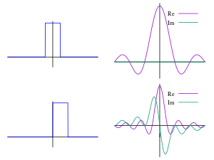
Fourier Transform
The original signal \(f(t)\) is shown on the left side and the real and imaginary components of its Fourier transform are plotted on the right.
Inverse Fourier Transform
The inverse Fourier transform of a function represents it using its component frequencies and their amplitudes.
Defn: The inverse Fourier transform of \(\hat{f}(\omega)\) of is
$$f(t) = \int _{-\infin}^{\infin} \hat{f}(\omega) e^{i \omega t} d \omega$$
Inverse Fourier Transform
Here we try to reconstruct square wave from coefficients using inverse Fourier transform.

Discrete Fourier Transforms
However, we often want to compute Fourier transforms on samples of an arbitrary function as opposed to on a symbolic representation. For this we use the discrete-time Fourier transform.
When the underlying signal is periodic, we can use the discrete Fourier transform instead of the discrete-time Fourier transform, which cannot be computed efficiently in general.
Discrete Fourier Transform
Defn: The discrete fourier transform (DFT) of a sequence of \(N\) complex numbers \(x_0, x_1, ..., x_{N-1}\) produces another sequence of complex numbers \(y_0, y_1, ..., y_{N-1}\) computed as follows:
$$y_k = \sum_{j=0}^{N-1} x_j e^{-i \omega jk}$$
where \(\omega = \frac{2 \pi}{N} = \) angular frequency of signal.
Discrete Fourier Transform
The input \(x_0, ..., x_{N-1}\) is the sequence of samples where \(x_k\) is the value of the signal at time \(k \Delta t\), \(\Delta t\) being the space between samples.
The output \(y_0, ..., y_N-1\) is the sequence of complex coefficients where \(y_k\) is the contribution from \(e^{i \omega k}\) to the signal.
Inverse Discrete Fourier Transform
Defn: The inverse discrete fourier transform of a sequence of \(N\) complex numbers \(y_0, y_1, ..., y_{N-1}\) produces another sequence of complex numbers \(x_0, x_1, ..., x_{N-1}\) computed as follows:
$$x_j = \frac{1}{N} \sum_{k=0}^{N-1} y_k e^{i \omega jk}$$
Quantum Fourier Transform
Important Properties of Fourier Transforms
Fourier transforms are:
- Linear
- Invertible
- Preserving of orthogonality
...sounds like a unitary transformation!
Setup
With \(n\) qubits in superposition, we have a state space
\(\{|00...0>, |00...1>, ..., |11...1>\}\) of size \(2^n\).
Let \(N = 2^n\) be the number of samples. If we apply the QFT on a register of \(n\) qubits in the state
$$|x> = x_0|0> + ... + x_{N-1}|N-1>$$ and get the state
$$|y> = QFT|x> = y_0|0> + ... + y_{N-1}|N-1>$$
we compute the DFT from \(\vec{x}\) to \(\vec{y}\).
QFT Formulation
Defn: The quantum Fourier transform from \(x_0, ..., x_N-1\) to \(y_0, ..., y_N-1\) is:
$$y_k = \frac{1}{\sqrt{N}} \sum_{j=0}^{N-1} x_j e^{i \omega jk}$$
where again \(\omega = \frac{2 \pi}{N}\).
The leading \(\frac{1}{\sqrt{N}}\) is to normalize the output state so that the QFT is unitary.
Inverse QFT
Defn: The inverse quantum Fourier transform from \(y_0, ..., y_N-1\) to \(x_0, ..., x_N-1\) is:
$$x_j = \frac{1}{\sqrt{N}} \sum_{k=0}^{N-1} y_k e^{-i \omega jk}$$
Since in the \(e^{i \omega jk}\) is a rotation, we just do the inverse rotation \(e^{-i \omega jk}\) in the inverse QFT.
Matrix Representation
The QFT can also be represented by a unitary matrix derived from the formula shown earlier
\begin{pmatrix}
1 & 1 & 1 & ... & 1 \\
1 & e^{i \omega} & e^{2i \omega} & ... & e^{i(N-1) \omega} \\
1 & e^{2i \omega} & e^{4i \omega} & ... & e^{2i(N-1) \omega} \\
. & . & . & & . \\
. & . & . & & . \\
. & . & . & & . \\
1 & e^{i(N-1) \omega} & e^{2i(N-1) \omega} & ... & e^{i(N-1)(N-1)}
\end{pmatrix}
Example!
Example!
Let's compute \(QFT|01\rangle\).
QFT_4 = \frac{1}{\sqrt{4}}
\begin{pmatrix}
1 & 1 & 1 & 1 \\
1 & e^{i \omega} & e^{2i \omega} & e^{3i \omega} \\
1 & e^{2i \omega} & e^{4i \omega} & e^{6i \omega} \\
1 & e^{3i \omega} & e^{6i \omega} & e^{9i \omega} \\
\end{pmatrix}
First we find
Example!
QFT_4 = \frac{1}{2}
\begin{pmatrix}
1 & 1 & 1 & 1 \\
1 & i & -1 & -i \\
1 & -1 & 1 & -1 \\
1 & -i & -1 & i \\
\end{pmatrix}
And because \(\omega = \frac{2 \pi}{N} = \frac{2 \pi}{2^n} = \frac{2 \pi}{2^4} = \frac{\pi}{8}\)
Example!
QFT_4|10\rangle = \frac{1}{2}
\begin{pmatrix}
1 & 1 & 1 & 1 \\
1 & i & -1 & -i \\
1 & -1 & 1 & -1 \\
1 & -i & -1 & i \\
\end{pmatrix}
\begin{pmatrix}
0 \\
0 \\
1 \\
0 \\
\end{pmatrix} \\
= \frac{1}{2}
\begin{pmatrix}
1 \\
-1 \\
1 \\
-1 \\
\end{pmatrix}
= \frac{1}{2}(|00\rangle - |01\rangle + |10\rangle - |11\rangle)
So,
Example!
This is exactly what we would expect since the Fourier transform of a delta function is sinusoidal.

So How is it Implemented on Real Hardware?
Circuit Implementation
We will use two operations to perform the QFT:
- Hadamard Gate
- Controlled Phase Gate
But just like in classical computing, to carry out a complex operation like the QFT, we must build it out of simpler gates that are easier to implement physically.
Strategy
The FFT computes the Fourier transform as follows:
$$\hat{f}(j) = (F_{N/2}\vec{f_{even}})(j) + e^{i \omega j}(F_{N/2}\vec{f_{odd}})(j)$$
Note that the Fourier transform \(F_N\) is an \(N \times N\) matrix.
Similarily we will take the QFT of the odd and even parts of the input sequence, and then multiply the odd terms by the phase \(e^{iwj}\).
Strategy
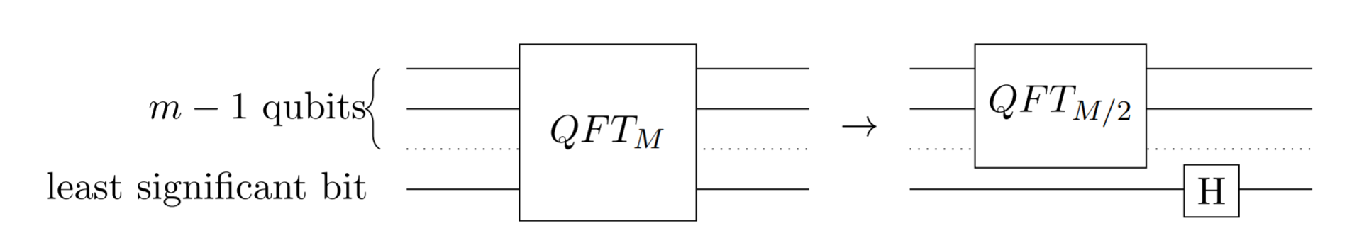
1. Attack subproblem - The odd and even terms are together in superposition. The odd terms are those whose least significant bit is 1, the even 0. Now we can apply \(QFT_{N/2}\) to the odd and even terms together by computing it on the \(n-1\) most significant bits.
2. Recombine - Since \(QFT_2 = H\) for a single qubit, after computing the QFT on the \(n-1\) most significant bits of that subproblem, we recombine by applying \(H\) on the least significant bit of that subproblem.
Strategy
Circuit diagram of \(QFT_M\) being split into subproblem and \(H\) gate.
Strategy
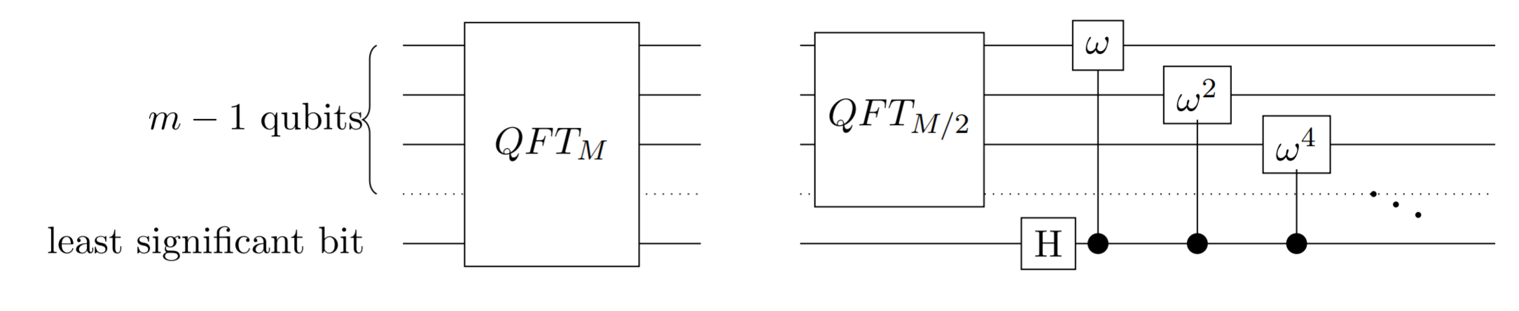
We apply this phase shift on all \(n-1\) most significant qubits.
We define \(\hat{R_k}\) to be the phase shift applied if the term is odd. The shift is applied on the \(k^{th}\) most significant bit of that subproblem:
3. Phase shift odd terms - Since we only want to phase shift odd terms, we use a controlled phase shift gate \(R_k\) whose control is the least significant bit. It will only phase shift the state when the least significant bit is 1 (the term is odd).
\hat{R}_k =
\begin{pmatrix}
1 & 0 \\
0 & e^{\frac{i \omega}{2^k}} \\
\end{pmatrix}
Strategy
Circuit diagram of full QFT on one subproblem.
Note: \(\omega = R_k\) controlled phase gate.
Example!
Let's compute \(QFT|x_1 x_2 x_3\rangle\).

Applications
Integer Factorization
Factoring numbers that have large prime factors is a difficult problem. The fastest classical algorithm for large numbers is called the general number field sieve, and runs in subexponential time
$$O(e^{1.9(logN)^{1/3}(loglogN)^{2/3}})$$ for an integer of size \(N\).
Many public-key cryptography schemes, including RSA, rely upon the assumption that integer factorization is difficult.
A 2,048 bit RSA key is computationally intractable on a classical computer, but with a large enough quantum computer it could be broken.

Shor's Factoring Algorithm
The algorithm has two steps:
- Turn factoring into a period finding problem (done classically)
- Find the period using the QFT
Runs in \(O(logN)^2(loglogN)(logloglogN))\) for integer of size \(N\).
Problem statement: Given an odd composite number \(N\), find an integer \(1 < d < N\) that divides \(N\).
Hidden Subgroup Problem
The HSP is a framework that captures problems like integer facorization, discrete logarithm, graph isomorphism, and the shortest vector problem.
Shor's algorithm solves the HSP on finite Abelian groups.
It is still an open question if efficient quantum algorithms exist for non-Abelian groups like the symmetric group (graph isomorphism) and dihedral group (shortest vector problem).
Solving Linear Systems
The Harrow Hassidim Lloyd (HLL) algorithm solves sparse linear systems with a low condition number \(\kappa\) (how sensitive output is to small changes in input) in \(O(log(N) \kappa^2)\) where \(N\) is the number of variables. The best classical algorithms take \(O(N \kappa)\).
Algorithm published in 2009, but first general-purpose implementation of the algorithm appeared in 2018 (Zhao et. al).
Uses quantum phase (eigenvalue) estimation which looks for an eigenvalue given an eigenvector and a unitary operator. Quantum phase estimation relies upon the inverse quantum Fourier transform as a subroutine.
Solving Linear Systems
Huge applications in science and engineering, from solving linear differential equations to machine learning.
Rebentrost et al. show that HLL can be used to provide an exponential speedup on quantum support vector machines.
In 2018, Zhao et. al developed an algorithm and included an implementation using HLL to perform Bayesian training of deep neural networks with exponential speedup.

I'd love to talk more and learn how quantum computing might make an impact in your field!
Stewy Slocum - sslocum3@jhu.edu
Quantum Fourier Transform and Applications
By Stewy Slocum


