Solving Equations
Numerical Methods
David Mayerich
Scalable Tissue Imaging and Modeling (STIM) Laboratory
Department of Electrical and Computer Engineering
Cullen College of Engineering
University of Houston
David Mayerich
STIM Laboratory, University of Houston

Solving Equations
Solving Equations Algebraically
Solving Quadratic Equations
Solutions as Roots
David Mayerich
STIM Laboratory, University of Houston
Solving Equations Algebraically
-
We often require the dependent variable \(x\) that satisfies an equation
David Mayerich
STIM Laboratory, University of Houston
y=f(x)
where the function \(f\) and \(y\) are known
-
This can be accomplished by calculating the inverse function:
x=f^{-1}(y)
Implementing Solutions
David Mayerich
STIM Laboratory, University of Houston
-
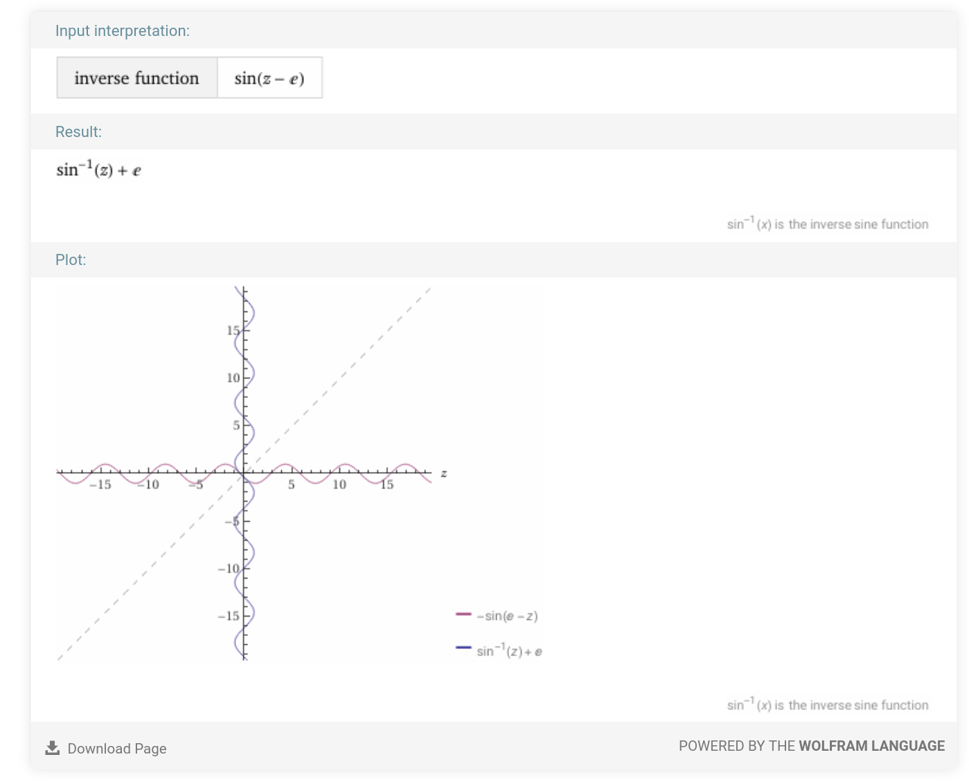
The inverse function \(f^{-1}(z)=\sin^{-1}(z) + e\) could be implemented as a series:
\sin^{-1}(x) = x + \frac{x^3}{6} + \frac{3x^5}{40} + O\left(x^6\right)
f^{-1}(z) \approx x + \frac{x^3}{6} + \frac{3x^5}{40} + e
-
Consider the equation: \(y = \sin(x - e)\)
\sin^{-1}(y) = x-e
\sin^{-1}(y) + e = x
f(z)=\sin(z-e)
f^{-1}(z)=\sin^{-1}(z) + e
Computer Algebra Systems
David Mayerich
STIM Laboratory, University of Houston
-
How can we get the inverse formulation: \(f(z)=\sin(z-e) \rightarrow f^{-1}(z)=\sin^{-1}(z) + e\)?
-
Computer Algebra Systems (CAS) can get us there:
-
Mathematica/Alpha (wolframalpha.com)
-
Symbolic Math Toolbox (MATLAB)
-
SymPy (sympy.org)
-
from sympy import *

y, z = symbols("y z")
solve(sin(z - exp(1)) - y, z)
[{z: asin(y) + E}, {z: -asin(y) + E + pi}]
Numerical Solutions
-
Consider functions without inverses
David Mayerich
STIM Laboratory, University of Houston
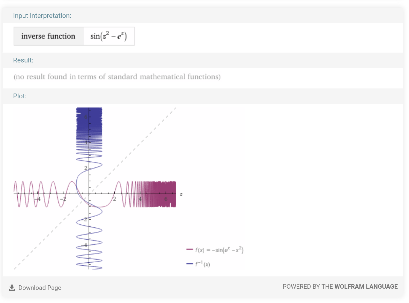
y = \sin\left(z^2 - e^z\right)
-
Wolfram Alpha cannot calculate the inverse but can generate a graph
-
This is done by expressing the equation as a root:
(the vast majority of them)
\sin\left(z^2 - e^z\right) - y = 0
-
Finding the roots of this equation for a given \(y\) gives the solution \(z\)
Root-Finding Formulas
-
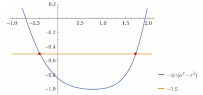
Find the solution to \(y = \sin\left(z^2 - e^z\right)\) for \(y = -0.5\)
David Mayerich
STIM Laboratory, University of Houston
\(z=-0.3909\)
-
Express the special functions as series:
\sin(z)\approx z
e^z \approx 1 + z + \frac{z^2}{2}
\sin\left(z^2 - e^z\right)\approx \frac{z^2}{2} - z - 1
\frac{z^2}{2} - z - 1 - y=0
\frac{1}{2}z^2 - z - 0.5=0
z=\frac{-b\pm \sqrt{b^2 - 4ac}}{2a}
z=\frac{1\pm \sqrt{(-1)^2 - 4(0.5)(-0.5)}}{2(0.5)}
=
[\ -0.4142,\ 2.414\ ]
\epsilon_r\approx 5.9\%
Simple Roots
David Mayerich
STIM Laboratory, University of Houston

-
Consider an interval \([a,b]\) of a function \(f(x)\in\mathbb{R}\) where \(f(a)\) and \(f(b)\) have opposite signs:
f(a)\cdot f(b) < 0
-
If \(f(x)\) is continuous on \([a,b]\), then there exists a number \(c\in[a,b]\) such that \(f(c)=0\)
-
The value \(x=c\) is a simple root of \(f\)
Bisection Method
Binary Searches for Roots
Bisection Algorithm
Error
David Mayerich
STIM Laboratory, University of Houston
Bisection Method
David Mayerich
STIM Laboratory, University of Houston
a
c
b
y=0
Bisection Method
David Mayerich
STIM Laboratory, University of Houston
y=0
a
b
c
Bisection Method
David Mayerich
STIM Laboratory, University of Houston
y=0
a
b
c
Bisection Method
David Mayerich
STIM Laboratory, University of Houston
y=0
a
b
c
Bisection Method
David Mayerich
STIM Laboratory, University of Houston
y=0
a
b
c
Bisection Method
David Mayerich
STIM Laboratory, University of Houston
y=0
a
b
c
Bisection Method
David Mayerich
STIM Laboratory, University of Houston
y=0
f(c) \approx 0
Bisection Method Evaluation
-
Calculate the solution to \(y=\sin\left(x^2 - e^x\right)\) for \(y=-0.5\) given the interval \([-1.0, -0.1]\) out to \(4\) digits of precision
David Mayerich
STIM Laboratory, University of Houston
\sin\left(x^2-e^x\right) = -0.5
-0.5500
0.2290
-0.3250
-0.07851
-0.4375
0.06122
-0.3813
-0.01206
-0.4094
0.0237015
-0.3954
0.005665
-0.3884
-0.003190
-0.3919
0.001224
-0.3902
-0.0009235
-0.3911
0.0002126
-0.3907
-0.0002925
-0.3909
-0.00004002
-1.000
1.091
-0.1000
-0.2801
-0.5500
0.2290
-0.1000
-0.2801
-0.5500
0.2290
-0.3250
-0.07851
-0.4375
0.06122
-0.3250
-0.07851
-0.4375
0.06122
-0.3813
-0.01206
-0.4094
0.0237015
-0.3813
-0.01206
-0.3954
0.005665
-0.3813
-0.01206
-0.3954
0.005665
-0.3884
-0.003190
-0.3919
0.001224
-0.3884
-0.003190
-0.3919
0.001224
-0.3902
-0.0009235
-0.3911
0.0002126
-0.3902
-0.0009235
-0.3911
0.0002126
-0.3907
-0.0002925
\sin\left(x^2-e^x\right)+0.5 = 0
\mathbf{a}
\mathbf{b}
\mathbf{f(a)}
\mathbf{f(b)}
\mathbf{c}
\mathbf{f(c)}
Bisection Method Algorithm
David Mayerich
STIM Laboratory, University of Houston
// implement the bisection method where:
// f is a function pointer that takes a parameter x and returns a value
// a and b are brackets bounding a root
// N is the maximum number of iterations
// return an approximation to the root bounded by a and b
double bisection(double (*f)(double), double a, double b, int N){
  float c;

  return c; // return the last approximation to the root
}
Bisection Method Algorithm
David Mayerich
STIM Laboratory, University of Houston
// implement the bisection method where:
// f is a function pointer that takes a parameter x and returns a value
// a and b are brackets bounding a root
// N is the maximum number of iterations
// return an approximation to the root bounded by a and b
double bisection(double (*f)(double), double a, double b, int N){
  float c;
  for(int i = 0; i < N; i++){ // iterate N times

  }
  return c; // return the last approximation to the root
}
Bisection Method Algorithm
David Mayerich
STIM Laboratory, University of Houston
// implement the bisection method where:
// f is a function pointer that takes a parameter x and returns a value
// a and b are brackets bounding a root
// N is the maximum number of iterations
// return an approximation to the root bounded by a and b
double bisection(double (*f)(double), double a, double b, int N){
  float c;
  for(int i = 0; i < N; i++){ // iterate N times
    c = (a + b) / 2.0; // find midpoint to approximate f(c) = 0
    if(f(c) == 0) return c; // if f(c) actually IS zero, return it (rare)
    if(f(a) * f(c) > 0) a = c; // if f(c) has the same sign as f(a), move a
    else b = c; // otherwise move b
  }
  return c; // return the last approximation to the root
}
Bisection Method - Example
-
Calculate the solution to \(y=\sin\left(x^2 - e^x\right)\) for \(y=-0.5\) given the interval \([-1.9, 1.7]\)
David Mayerich
STIM Laboratory, University of Houston
double func(double z) {
	return = sin(z*z - exp(z));
}
Bisection Method - Example
-
Calculate the solution to \(y=\sin\left(x^2 - e^x\right)\) for \(y=-0.5\) given the interval \([-1.9, 1.7]\)
David Mayerich
STIM Laboratory, University of Houston
double func(double z) {
	return = sin(z*z - exp(z));
}

int main(int argc, char** argv) {
	int N = 100;

    double result = bisection(func, -1.9, 1.7, N);

}
Bisection Method Theorem
If the bisection method is applied to a continuous function \(f\) on an interval \([a, b]\), where \(f(a)f(b)<0\), then after \(n\) steps an approximate root will be computed with an error at most \(\epsilon = \frac{b-a}{2^n}\).
David Mayerich
STIM Laboratory, University of Houston
-
Each iteration computes the root with one additional binary bit of precision
-
How many iterations are required to guarantee an error less than \(\epsilon'\)?
\frac{b-a}{2^n} < \epsilon'
b-a < 2^n \epsilon'
\log(b-a) < n \log 2 + \log \epsilon'
\log(b-a) - \log \epsilon' < n \log 2
n > \frac{\log(b-a) - \log \epsilon'}{\log 2}
n = \left\lceil\frac{\log(b-a) - \log \epsilon'}{\log 2}\right\rceil
Bisection Method Characteristics
-
Very robust - guaranteed to converge to a root as long as \(f(a)f(b)<0\)
-
Does not work for multiple roots when \(f(a)f(b) \geq 0\)
-
Binary search reduces error by \(O(2^n)\) after \(n\) iterations
-
This is equivalent to \(1\) bit per iteration
-
\(\approx 23\) iterations for
float, \(\approx 53\) iterations fordouble
-
David Mayerich
STIM Laboratory, University of Houston
Method of False Position
Combining Function Size and Magnitude
Method of False Position Algorithm
Problems
David Mayerich
STIM Laboratory, University of Houston
Method of False Position
David Mayerich
STIM Laboratory, University of Houston
a
c
b
y=0
Method of False Position
David Mayerich
STIM Laboratory, University of Houston
a
c
b
y=0
Method of False Position
David Mayerich
STIM Laboratory, University of Houston
a
c
b
y=0
Method of False Position
-
Instead of using the midpoint for \(c\), use the x-intercept of \(\overline{f(a)f(b)}\)
-
Given the bracket \([a, b]\), we calculate two points: \(\left( a, f(a)\right)\) and \(\left( b, f(b)\right)\)
-
The line between them is specified by:
David Mayerich
STIM Laboratory, University of Houston
y=mx+b
y(x)=\frac{f(a)-f(b)}{b-a} (x-a) + f(a)
-
Setting \(y(x)=0\) and simplifying yields the root of the line at:
x=\frac{a f(b) - b f(a)}{f(b)-f(a)}
Method of False Position Algorithm
David Mayerich
STIM Laboratory, University of Houston
// implement the method of false position where:
// f is a function pointer that takes a parameter x and returns a value
// a and b are brackets bounding a root
// N is the maximum number of iterations
// return an approximation to the root bounded by a and b
double mfp(double (*f)(double), double a, double b, int N){
  double c;

  return c; // return the last approximation to the root
}
Method of False Position Algorithm
David Mayerich
STIM Laboratory, University of Houston
// implement the method of false position where:
// f is a function pointer that takes a parameter x and returns a value
// a and b are brackets bounding a root
// N is the maximum number of iterations
// return an approximation to the root bounded by a and b
double mfp(double (*f)(double), double a, double b, int N){
  double c;
  for(int i = 0; i < N; i++){ // iterate N times

  }
  return c; // return the last approximation to the root
}
Method of False Position Algorithm
David Mayerich
STIM Laboratory, University of Houston
// implement the method of false position where:
// f is a function pointer that takes a parameter x and returns a value
// a and b are brackets bounding a root
// N is the maximum number of iterations
// return an approximation to the root bounded by a and b
double mfp(double (*f)(double), double a, double b, int N){
  double c;
  for(int i = 0; i < N; i++){ // iterate N times
    double fa = f(a); // precompute f(a) and f(b)
    double fb = f(b);
    c = (a * fb – b * fa) / (fb – fa);// WAS (a + b) / 2
    if(f(c) == 0) return c; // if f(c) actually IS zero, return it (rare)
    if(f(a) * f(c) > 0) a = c; // if f(c) has the same sign as f(a), move a
    else b = c; // otherwise move b
  }
  return c; // return the last approximation to the root
}
Bracketing Convergence
Convergence Analysis
Bisection and False Position
David Mayerich
STIM Laboratory, University of Houston
Bisection Method Behavior
-
What we know given the bracket \([a, b]\) on a continuous function \(f(x)\) if \(a \leq b\):
-
At each iteration \(n\), the update for \(a_n\) will always increase:
\(a\rightarrow a_0 \leq a_1 \leq a_2 \leq \cdots \leq a_n\) -
At each iteration \(n\), the update for \(b_n\) will always decrease:
\(b\rightarrow b_0 \geq b_1 \geq b_2 \geq \cdots \geq b_n\) -
As \(n\) increases, we expect both sides of the bracket to converge to the root \(r\):
-
From the Bisection Method Theorem, we know that:
-
David Mayerich
STIM Laboratory, University of Houston
\lim_{n\rightarrow \infty} a_n
=
\lim_{n\rightarrow \infty} b_n
=
r
b_n - a_n = \frac{b_0 - a_0}{2^n}
Bisection Convergence Rate
-
For any iteration \(n\geq 1\), the Bisection Method calculates a new value \(c_n\):
David Mayerich
STIM Laboratory, University of Houston
|r - c_n| \leq \frac{b_n - a_n}{2} = \frac{b - a}{2^n}
|r - c_n| \leq \left( \frac{1}{2} \right)^n |b-a|
-
The convergence rate specifies how quickly the error reduces across iterations:
\lim_{n\rightarrow\infty} \frac{|r - c_n|}{|r-c_{n-1}|}
=
\frac{\left(\frac{1}{2}\right)^{n}|b-a|}{\left(\frac{1}{2} \right)^{n-1}|b-a|}
=
\frac{\left(\frac{1}{2}\right)^{n}}{\left(\frac{1}{2} \right)^{n-1}}
=
\frac{1}{2}
D.1 Bracketing Methods
By STIM Laboratory


