Regression
Numerical Methods
David Mayerich
Scalable Tissue Imaging and Modeling (STIM) Laboratory
Department of Electrical and Computer Engineering
Cullen College of Engineering
University of Houston
David Mayerich
STIM Laboratory, University of Houston

A Review of Vector Norms
-
The norm provides a measure of the magnitude of a vector
-
The notation \(||\mathbf{x}||_p\) denotes the \(L^p\) norm of a vector:
David Mayerich
STIM Laboratory, University of Houston
||\mathbf{x}||_p = \sqrt[p]{\sum_{i=1}^n |x_i|^p}
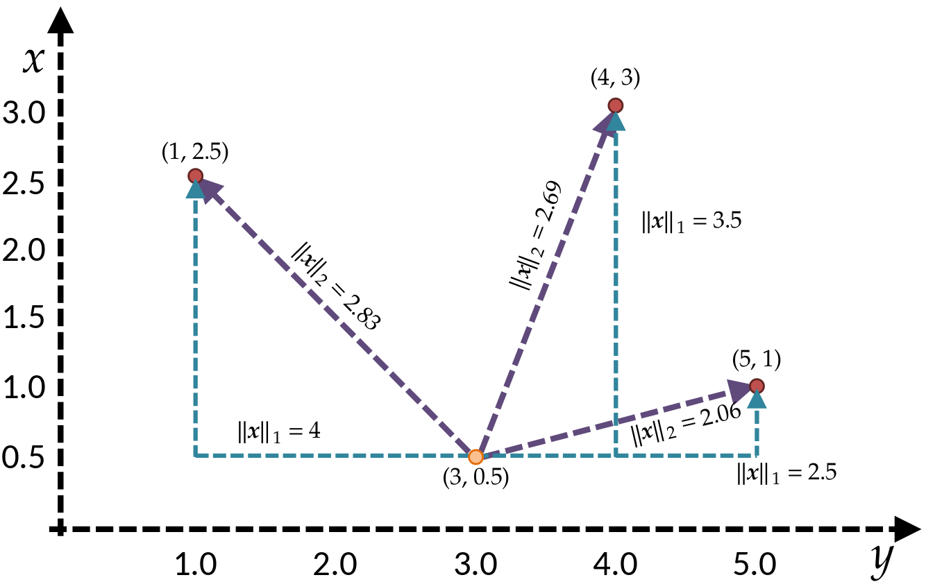
||\mathbf{x}||_1 = \sum_{i=1}^n |x_i|
Manhattan
||\mathbf{x}||_2 = \sqrt{\sum_{i=1}^n x_i^2}
Euclidean
Statistics
-
Common statistical measurements of a vector \(\mathbf{x}\in\mathbb{R}^n\) include:
-
mean, average, or expected value:
David Mayerich
STIM Laboratory, University of Houston
-
variance:
-
standard deviation:
\mu(\mathbf{x}) = E[\mathbf{x}] = \frac{1}{n}\sum_{i=0}^n x_i
\sigma^2(\mathbf{x}) = \frac{1}{n}\sum_{i=0}^n \left[x_i - \mu(\mathbf{x})\right]^2
\sigma(\mathbf{x}) = \sqrt{\sigma^2(\mathbf{x})}
\mathbf{x} = \{10, 20, 30, 40, 50\}
\mathbf{y} = \{30, 30, 30, 30, 30\}
\mu(\mathbf{x}) = 30
\mu(\mathbf{y}) = 30
\sigma^2(\mathbf{x}) = 200
\sigma^2(\mathbf{y}) = 0
\sigma(\mathbf{x}) = 14.14
\sigma(\mathbf{y}) = 0
Regression
-
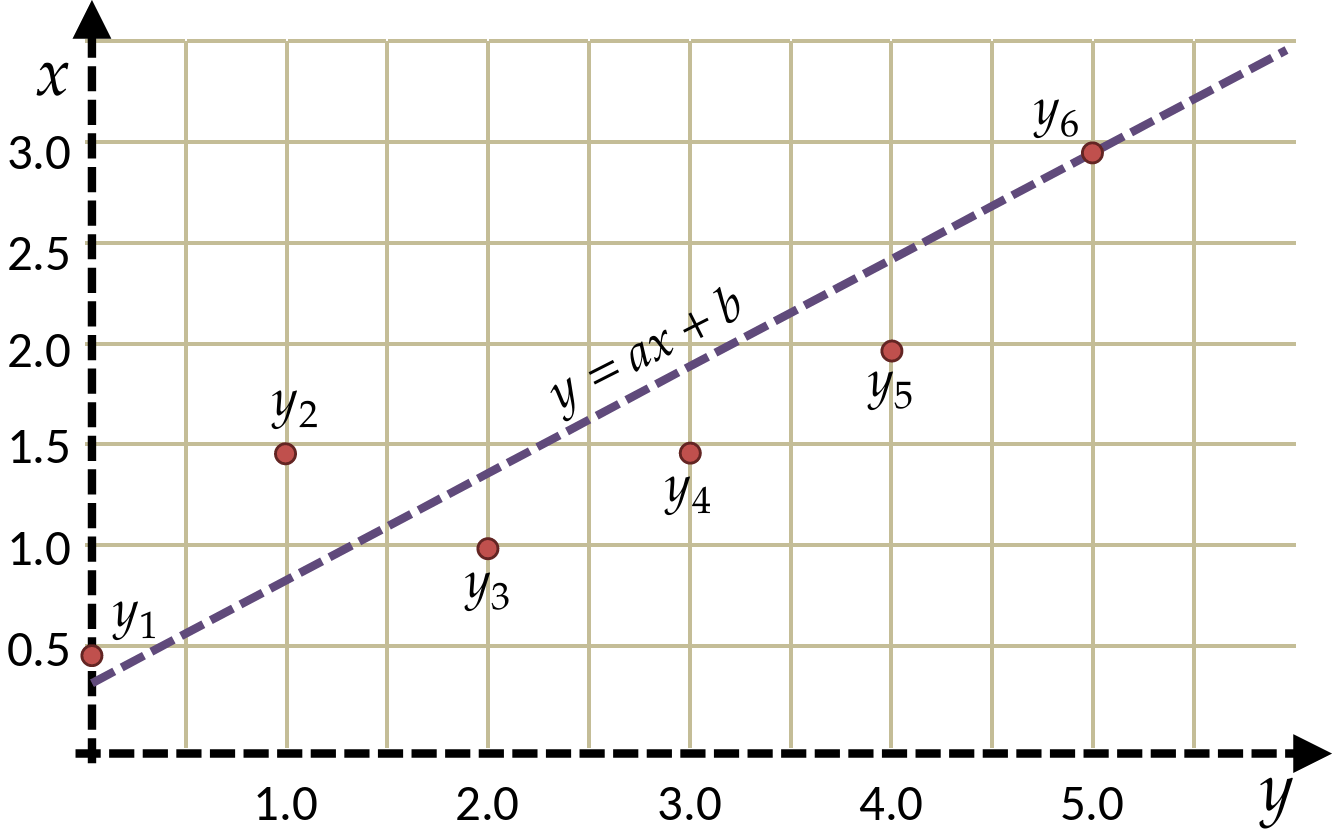
Assume we have a table of data points containing \((x_i,y_i)\) pairs
-
Prior information suggests that these points are on a line
-
(deviations may be due to noise, measurement errors, etc.)
-
David Mayerich
STIM Laboratory, University of Houston
| x | y |
|---|---|
| 0.0 | 0.5 |
| 1.0 | 1.5 |
| 2.0 | 1.0 |
| 3.0 | 1.5 |
| 4.0 | 2.0 |
| 5.0 | 3.5 |
Regression
-
How can we approximate this known function from measured points?
-
If we know that the expected model is a line:
David Mayerich
STIM Laboratory, University of Houston
y(x)=ax+b
where \(a\) and \(b\) are the parameters we want to know
-
If we plug in some value \(x_i\) and our model is accurate, we expect:
ax_i+b \approx y_i
or, alternatively
ax_i+b - y_i = \epsilon
-
We want the error term \(\epsilon\) to be as small as possible
Regression Error
-
We calculate the absolute error for a single value:
David Mayerich
STIM Laboratory, University of Houston
\epsilon_i = |ax_i+b - y_i|
-
The sum of all absolute errors gives us a metric to quantify the "fit" between our model and the points:
\epsilon_s = \sum_{i=1}^n |ax_i+b - y_i|
= ||a\mathbf{x} + b - \mathbf{y}||_1
-
We could select \(a\) and \(b\) such that the \(L^1\) norm is minimized
-
Unfortunately \(L^1\) minimization is difficult:
-
Finding minima of functions generally relies on solving a differential equation
-
\(||\mathbf{x}||_1\) is not differentiable
-
Minimization of Error
-
We have a set of observations:
David Mayerich
STIM Laboratory, University of Houston
B = \{(x_1, y_1), (x_2, y_2), \cdots, (x_n, y_n)\}
-
We can look at the set of values describing the difference between our model \(y=ax+b\) and the observations \(B\):
\Psi = \{(ax_1+b-y_1), (ax_2 + b - y_2), \cdots, (ax_n + b - y_n)\}
-
What characteristics do we expect in \(\Psi\) if \(a\) and \(b\) are good parameters?
-
The mean \(\mu(\Psi)\) will be small:
-
all points will lie on the line OR some points will lie above and some below
-
- The variance \(\sigma^2(\Psi)\) will describe the quality of the fit
- ideally \(\sigma^2(\Psi)\) will be small (\(\sigma^2(\Psi) = 0\) if all points are on the line)
Minimization of Error
-
Note that the mean of the difference between the model and the measurements are given by:
David Mayerich
STIM Laboratory, University of Houston
\mu(\Psi) = \frac{1}{n}\sum_{i=1}^n |ax_i+b - y_i|
-
With a small mean (\(\mu\approx 0\)), the variance is:
\sigma^2(\Psi) \approx \frac{1}{n}\sum_{i=1}^n |ax_i+b - y_i|^2
-
What happens to our line if we select \(a\) and \(b\) such that the variance is minimized?
-
Minimizing the variance \(\sigma^2(\Phi)\) minimizes deviation between the model and the measurements
Cost Functions
-
A cost function can be used to describe the quality of a set of parameters
-
The cost function \(K(\cdots)\) is a function of parameters we are searching for:
David Mayerich
STIM Laboratory, University of Houston
model
cost function
y=ax+b
K(a, b) = \cdots
-
A smaller value defines a better fit than a larger value:
if \(K(a_1, b_1)<K(a_2, b_2)\) then \(a_1\) and \(b_1\) are "better" parameters
-
It is helpful to have a cost function that is differentiable
-
ex. you can find local minima with Newton's method
-
if a cost function can't be differentiated, we have to use a more complex optimization
-
Cost Functions
-
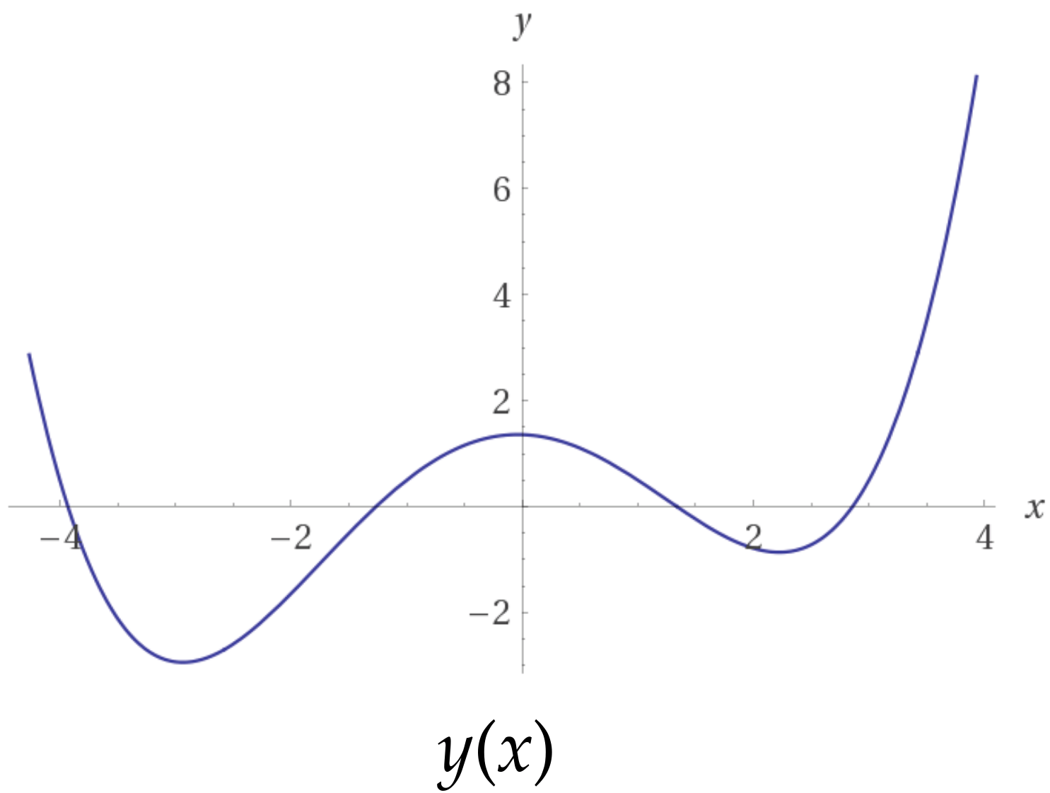
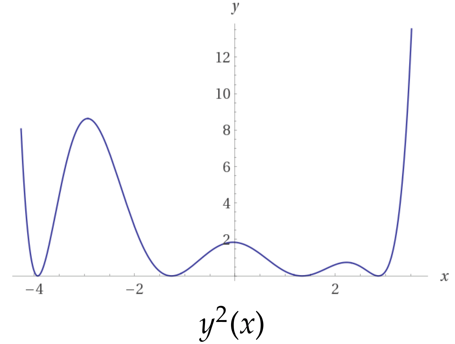
You've worked with cost functions before
-
Finding a root \(f(x)\) be expressed as a cost function \(f^2(x)\)
David Mayerich
STIM Laboratory, University of Houston
Least Squares Fitting
-
Create a model function \(y(x)\) that minimizes the square of the difference between \(y(x)\) and at the points \((x_i, y_i)\)
David Mayerich
STIM Laboratory, University of Houston
K(a, b) \approx \sum_{i=1}^n [ax_i+b - y_i]^2
-
Linear least squares fitting:
-
the model function is linear in terms of the parameters (\(a, b, \cdots\))
-
the functions \(y_1(x), y_2(x), \cdots\) do not have to be linear - only the coefficients
-
why would this be useful?
-
the cost function is quadratic: there is only one minimum
-
y(x)=ay_1(x) + by_2(x)+cy_3(x) + \cdots
Designing a Cost Function for a Line
-
The variance of the difference between \(N\) measured points and \(y(x)\) is:
David Mayerich
STIM Laboratory, University of Houston
y(x)=ax+b
\sigma^2(\Phi)=\frac{1}{n} \sum_{i=1}^n (ax_i + b - y_i)^2
-
Create a cost function \(K\):
K(a, b)=\sum_{i=1}^n (ax_i + b - y_i)^2 = n \cdot \sigma^2(\Phi)
-
It doesn't matter if we minimize the variance, or \(N\) times the variance
(the minimum values have the same \(x\) coordinates) -
\(K\) is differentiable and quadratic: it only has one global minimum
Find the Minimum of the Cost Function
-
Since \(K\) is a quadratic function, there is only one minimum characterized by:
David Mayerich
STIM Laboratory, University of Houston
K(a, b)=\sum_{i=1}^n (ax_i + b - y_i)^2
\frac{dK}{da}=0
\frac{dK}{db}=0
-
Find the set of linear equations for the optimal \(a\) and \(b\):
\frac{d}{da}K(a, b)=\sum_{i=1}^n 2(ax_i + b - y_i)x_i
\frac{d}{db}K(a, b)=\sum_{i=1}^n 2(ax_i + b - y_i)
\frac{d}{da}K(a, b)=\sum_{i=1}^n (ax_i + b - y_i)x_i = 0
\frac{d}{db}K(a, b)=\sum_{i=1}^n (ax_i + b - y_i) = 0
Find the Minimum of the Cost Function
-
This leaves us with two linear equations to solve:
David Mayerich
STIM Laboratory, University of Houston
\sum_{i=1}^n (ax_i + b - y_i)x_i = 0
\sum_{i=1}^n (ax_i + b - y_i) = 0
\sum_{i=1}^n (ax_i^2 + bx_i - y_ix_i) = 0
\sum_{i=1}^n ax_i^2 + \sum_{i=1}^n bx_i = \sum_{i=1}^n y_ix_i
\sum_{i=1}^n ax_i + \sum_{i=1}^n b = \sum_{i=1}^n y_i
\sum_{i=1}^n ax_i + n \cdot b = \sum_{i=1}^n y_i
Solve the Linear System
David Mayerich
STIM Laboratory, University of Houston
\sum_{i=1}^n ax_i^2 + \sum_{i=1}^n bx_i = \sum_{i=1}^n y_ix_i
\sum_{i=1}^n ax_i + n \cdot b = \sum_{i=1}^n y_i
\begin{bmatrix}
\sum_{i=1}^n x_i^2 &
\sum_{i=1}^n x_i \\
\sum_{i=1}^n x_i &
N
\end{bmatrix}
\begin{bmatrix}
a\\
b
\end{bmatrix}
=
\begin{bmatrix}
\sum_{i=1}^n y_ix_i\\
\sum_{i=1}^n y_i
\end{bmatrix}
Stability
-
The determinant of a \(2\times 2\) matrix \(\mathbf{M}\) is:
David Mayerich
STIM Laboratory, University of Houston
\text{det}\begin{bmatrix}
a & b\\
c & d
\end{bmatrix}
=
ad - bc
-
The matrix used in linear least squares is:
\mathbf{M}=\begin{bmatrix}
\sum_{i=1}^n x_i^2 &
\sum_{i=1}^n x_i \\
\sum_{i=1}^n x_i &
N
\end{bmatrix}
-
So the determinant is given by:
|\mathbf{M}| =
N\sum_{i=1}^n x_i^2
-
\left(
\sum_{i=1}^n x_i
\right)^2
-
Since the mean of \(\mathbf{x}\) is:
\mu(\mathbf{x})=\frac{1}{n}\sum_{i=1}^n x_i
-
The determinant can be simplified to:
|\mathbf{M}| =
N\sum_{i=1}^n x_i^2
-
(n\mu(\mathbf{x}))^2
=
n^2(\mu(\mathbf{x}^2)-\mu^2(\mathbf{x}))
-
The determinant is zero when \(\mu(\mathbf{x}^2)=\mu^2(\mathbf{x})\)
when all \(x_i\) values are identical
F.2 Regression
By STIM Laboratory


