Properties of Linear Systems
Numerical Methods
David Mayerich
Scalable Tissue Imaging and Modeling (STIM) Laboratory
Department of Electrical and Computer Engineering
Cullen College of Engineering
University of Houston
David Mayerich
STIM Laboratory, University of Houston

Matrix Inversion
David Mayerich
STIM Laboratory, University of Houston
Matrix Inverse
-
Some applications require calculating the matrix inverse \(\mathbf{A}^{-1}\)
-
Computer graphics, image processing, multiple-input multiple-output (MIMO) communication
-
Determining if a linear system is ill-conditioned
-
-
By definition, the matrix inverse is:
David Mayerich
STIM Laboratory, University of Houston
\mathbf{Ax}=\mathbf{b}
\mathbf{A}^{-1}\mathbf{A}\mathbf{x}=\mathbf{A}^{-1}\mathbf{b}
\mathbf{x}=\mathbf{A}^{-1}\mathbf{b}
\mathbf{A}^{-1}\mathbf{A}=\mathbf{A}\mathbf{A}^{-1}=\mathbf{I}
\mathbf{LU}\mathbf{A}^{-1}=\mathbf{I}
Invert by LU Decomposition
David Mayerich
STIM Laboratory, University of Houston
\mathbf{A}=
\begin{bmatrix}
1 & 0 & 2\\
2 & -1 & 3\\
4 & 1 & 8
\end{bmatrix}
\mathbf{L}_0=
\begin{bmatrix}
1 & 0 & 0\\
0 & 1 & 0\\
0 & 0 & 1
\end{bmatrix}
\mathbf{U}_0=
\begin{bmatrix}
1 & 0 & 2\\
2 & -1 & 3\\
4 & 1 & 8
\end{bmatrix}
\mathbf{L}_1=
\begin{bmatrix}
1 & 0 & 0\\
2 & 1 & 0\\
4 & 0 & 1
\end{bmatrix}
\mathbf{U}_1=
\begin{bmatrix}
1 & 0 & 2\\
0 & -1 & -1\\
0 & 1 & 0
\end{bmatrix}
\mathbf{L}=
\begin{bmatrix}
1 & 0 & 0\\
2 & 1 & 0\\
4 & -2 & 1
\end{bmatrix}
\mathbf{U}=
\begin{bmatrix}
1 & 0 & 2\\
0 & -1 & -1\\
0 & 0 & -1
\end{bmatrix}
Invert by LU Decomposition
David Mayerich
STIM Laboratory, University of Houston
\mathbf{A}=
\begin{bmatrix}
1 & 0 & 2\\
2 & -1 & 3\\
4 & 1 & 8
\end{bmatrix}
\mathbf{L}=
\begin{bmatrix}
1 & 0 & 0\\
2 & 1 & 0\\
4 & -2 & 1
\end{bmatrix}
\mathbf{U}=
\begin{bmatrix}
1 & 0 & 2\\
0 & -1 & -1\\
0 & 0 & -1
\end{bmatrix}
\begin{bmatrix}
1 & 0 & 0\\
2 & 1 & 0\\
4 & -2 & 1
\end{bmatrix}
\begin{bmatrix}
1 & 0 & 2\\
0 & -1 & -1\\
0 & 0 & -1
\end{bmatrix}
\begin{bmatrix}
a_{11} & a_{12} & a_{13}\\
a_{21} & a_{22} & a_{23}\\
a_{31} & a_{32} & a_{33}
\end{bmatrix}
=
\begin{bmatrix}
1 & 0 & 0\\
0 & 1 & 0\\
0 & 0 & 1
\end{bmatrix}
\mathbf{b}_1 =
\begin{bmatrix}
1\\
0\\
0
\end{bmatrix}
\mathbf{b}_2 =
\begin{bmatrix}
0\\
1\\
0
\end{bmatrix}
\mathbf{b}_3 =
\begin{bmatrix}
0\\
0\\
1
\end{bmatrix}
\mathbf{a}_1 =
\begin{bmatrix}
-11\\
-4\\
6
\end{bmatrix}
\mathbf{a}_2 =
\begin{bmatrix}
2\\
0\\
-1
\end{bmatrix}
\mathbf{a}_3 =
\begin{bmatrix}
2\\
1\\
-1
\end{bmatrix}
\mathbf{A}^{-1} =
\begin{bmatrix}
-11 & 2 & 2\\
-4 & 0 & 1\\
6 & -1 & -1
\end{bmatrix}
Singular Matrices
Infinite or no solutions
Determinants
David Mayerich
STIM Laboratory, University of Houston
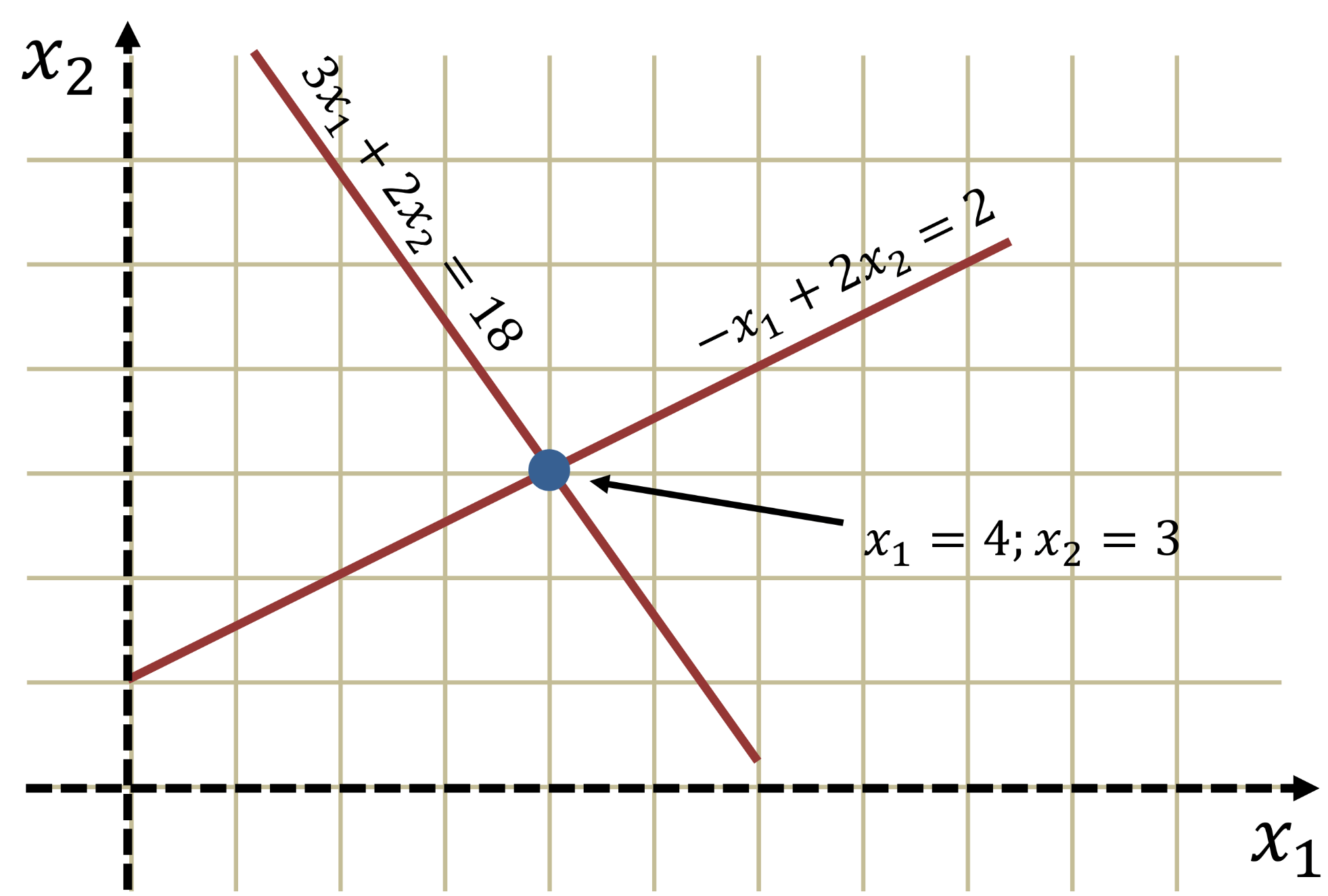
Linear Systems Graphically
-
Given the linear system:
David Mayerich
STIM Laboratory, University of Houston
3x_1 + 2x_2 = 18
-x_1 + 2x_2 = 2
The solution is the intersection of both lines:
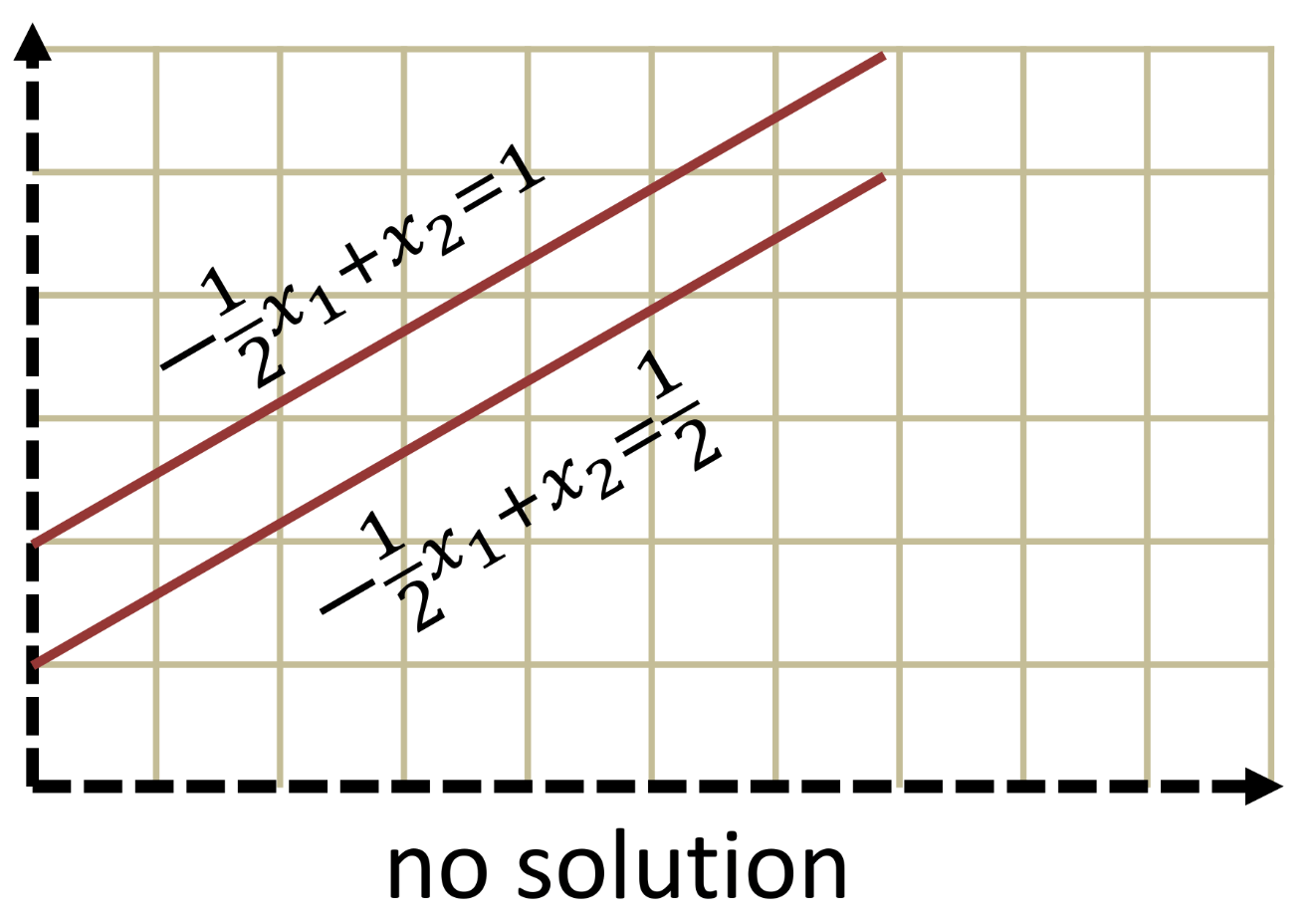
Singular Matrices
-
Singular matrices do not have a unique solution
-
Parallel planes indicate that the system has no solution
-
Overlapping planes result in infinite solutions
-
David Mayerich
STIM Laboratory, University of Houston
-
Matrices with multiple solutions or no solutions
- Statistically these are rare (if you generate random matrices)

Determinants
David Mayerich
STIM Laboratory, University of Houston
\text{det}
\begin{bmatrix}
a_{11} & a_{12}& \cdots & a_{1n}\\
a_{21} & a_{22}& \cdots & a_{2n}\\
\vdots & \vdots & \ddots & a_{3n}\\
a_{n1} & a_{n2}& \cdots & a_{nn}
\end{bmatrix}
=
\begin{vmatrix}
a_{11} & a_{12}& \cdots & a_{1n}\\
a_{21} & a_{22}& \cdots & a_{2n}\\
\vdots & \vdots & \ddots & a_{3n}\\
a_{n1} & a_{n2}& \cdots & a_{nn}
\end{vmatrix}
-
Singular matrices can be found using the determinant:
-
Determinants of small matrices:
\text{det}
\begin{bmatrix}
a & b\\
c & d
\end{bmatrix}
=
ad-bc
\text{det}
\begin{bmatrix}
a_1 & a_2 & a_3\\
b_1 & b_2 & b_3\\
c_1 & c_2 & c_3
\end{bmatrix}
\begin{split}
&=
(a_1 b_2 c_3 + a_2 b_3 c_1 + a_3 b_1 c_2)\\
&-
(a_1 b_3 c_2 + a_2 b_1 c_3 + a_3 b_2 c_1)
\end{split}
Properties of Determinants
-
The determinant of the identity matrix is \(1\):
-
The determinant of the inverse of a matrix is equal to the inverse of the determinant:
-
Multiplication by a scalar value \(\alpha\):
-
The determinant of a matrix product is equal to the product of the determinants:
-
A linear system \(\mathbf{Ax}=\mathbf{b}\) has a unique solution if and only if \(\text{det}(\mathbf{A})\neq 0\)
David Mayerich
STIM Laboratory, University of Houston
\text{det}(\mathbf{I})=1
\text{det}(\mathbf{A}^{-1})=\frac{1}{\text{det}(\mathbf{A})}
\text{det}(\alpha\mathbf{A})=\alpha^n \text{det}(\mathbf{A}) \quad\text{where}\quad
\mathbf{A}\in \mathbb{R}^{n\times n}
\text{det}(\mathbf{AB})=
\text{det}(\mathbf{A})
\text{det}(\mathbf{B})
Laplace Expansion
-
For general matrices \(\mathbf{A}\in \mathbb{R}^{n \times n}\), the Laplace expansion can be used:
David Mayerich
STIM Laboratory, University of Houston
\text{det}(\mathbf{A}) =
\sum_{j=1}^{n}
(-1)^{i+j} a_{ij} |\mathbf{M}_{ij}|
\quad
\text{for any row } i
\(a_{ij}\) is the scalar entry at row \(i\) and column \(j\)
\(\mathbf{M}_{ij}\) is the submatrix of \(\mathbf{A}\) with row \(i\) and column \(j\) removed
-
Consider the Laplace expansion of a \(3\times 3\) matrix using row \(1\):
\mathbf{A} =
\begin{bmatrix}
2 & 4 & 6 \\
1 & 2 & 7 \\
2 & 8 & 2
\end{bmatrix}
\begin{vmatrix}
2 & 4 & 6 \\
1 & 2 & 7 \\
2 & 8 & 2
\end{vmatrix}
=
2
\begin{vmatrix}
2 & 7\\
8 & 2
\end{vmatrix}
-
4
\begin{vmatrix}
1 & 7\\
2 & 2
\end{vmatrix}
+
6
\begin{vmatrix}
1 & 2\\
2 & 8
\end{vmatrix}
=
2
(4 - 56)
-
4
(2 - 14)
+
6
(8 - 4)
=
-104
+
48
+
24
=
-32
The Laplace expansion is a recursive algorithm with non-polynomial complexity \(O(n!)\)
Laplace Expansions for Diagonal Matrices
-
Calculate the Laplace expansion for row \(2\) of the matrix:
David Mayerich
STIM Laboratory, University of Houston
\mathbf{A} =
\begin{bmatrix}
1 & 2 & 3\\
0 & 4 & 5\\
0 & 0 & 6
\end{bmatrix}
\text{det}(\mathbf{A}) =
\sum_{j=1}^{n}
(-1)^{i+j} a_{ij} |\mathbf{M}_{ij}|
\begin{vmatrix}
1 & 2 & 3\\
0 & 4 & 5\\
0 & 0 & 6
\end{vmatrix}
=
-0
\begin{vmatrix}
2 & 3\\
0 & 6
\end{vmatrix}
+
4
\begin{vmatrix}
1 & 3\\
0 & 6
\end{vmatrix}
-
5
\begin{vmatrix}
1 & 2\\
0 & 0
\end{vmatrix}
=4(1\cdot 6)=24
\begin{vmatrix}
a & b & c & d\\
0 & e & f & g\\
0 & 0 & h & i\\
0 & 0 & 0 & j
\end{vmatrix}
=
j\begin{vmatrix}
a & b & c\\
0 & e & f\\
0 & 0 & h
\end{vmatrix}
-
Calculate the Laplace expansion for row \(4\):
=
j
\left(
h
\begin{vmatrix}
a & b\\
0 & e
\end{vmatrix}
\right)
=
j
\left(
h(a \cdot e)
\right)
Calculating \(n\times n\) Determinants
-
The determinant of a triangular matrix is the product of the diagonal elements:
David Mayerich
STIM Laboratory, University of Houston
\text{det}
\begin{bmatrix}
a_{11} & a_{12}& \cdots & a_{1n}\\
0 & a_{22}& \cdots & a_{2n}\\
\vdots & \vdots & \ddots & a_{3n}\\
0 & 0 & \cdots & a_{nn}
\end{bmatrix}
=
a_{11} a_{22} \cdots a_{nn}
-
Given the product property \(|\mathbf{A}\mathbf{B}| = |\mathbf{A}| |\mathbf{B}|\), what is \(|\mathbf{A}| = |\mathbf{LU}|\)?
\text{det}(\mathbf{A}) = \text{det}(\mathbf{U})
-
The determinant of a matrix \(\mathbf{A}\) can be solved using LU decomposition and calculating the product of the diagonal of \(\mathbf{U}\)
Determinants with Pivoting
-
Swapping rows in a matrix \(\mathbf{A}\) multiplies the determinant by \((-1)\)
David Mayerich
STIM Laboratory, University of Houston
\mathbf{A} =
\begin{bmatrix}
2 & 6 & 6 \\
1 & 2 & 8 \\
2 & 8 & 2
\end{bmatrix}
-
Calculate the determinant using scaled partial pivoting:
\mathbf{U}_0 =
\begin{bmatrix}
2 & 4 & 6 \\
1 & 2 & 8 \\
2 & 8 & 2
\end{bmatrix}
\rightarrow
\begin{bmatrix}
1 & 2 & 8 \\
2 & 6 & 6 \\
2 & 8 & 2
\end{bmatrix}
\mathbf{U}_1 =
\begin{bmatrix}
1 & 2 & 8 \\
0 & 2 & -10 \\
0 & 4 & -14
\end{bmatrix}
\rightarrow
\begin{bmatrix}
1 & 2 & 8 \\
0 & 4 & -14 \\
0 & 2 & -10
\end{bmatrix}
\mathbf{U}_2 =
\begin{bmatrix}
1 & 2 & 8 \\
0 & 4 & -14 \\
0 & 0 & 17
\end{bmatrix}
|\mathbf{A}| = 1 \cdot 4 \cdot 17 \cdot (-1)\cdot (-1)
= 68
swap
swap
Matrix Norms
Euclidean and Manhattan Distance
Matrix and Vector Norms
David Mayerich
STIM Laboratory, University of Houston
Vector Norms
-
A vector norm is a scalar metric used to calculate the length of a vector
-
The most common set of vector norms are the \(L^p\)-norms:
David Mayerich
STIM Laboratory, University of Houston
||\mathbf{v}||_p=
\left(
\sum_{i=1}^N
|v_i|^p
\right)
^{\frac{1}{p}}
=
\sqrt[p]{
\sum_{i=1}^N
|v_i|^p
}
-
The two most common are the \(L^2\)-norm and \(L^1\)-norm:
||\mathbf{v}||_2=
\sqrt{
\sum_{i=1}^N
v_i^2
}
||\mathbf{v}||_1=
\sum_{i=1}^N
|v_i|
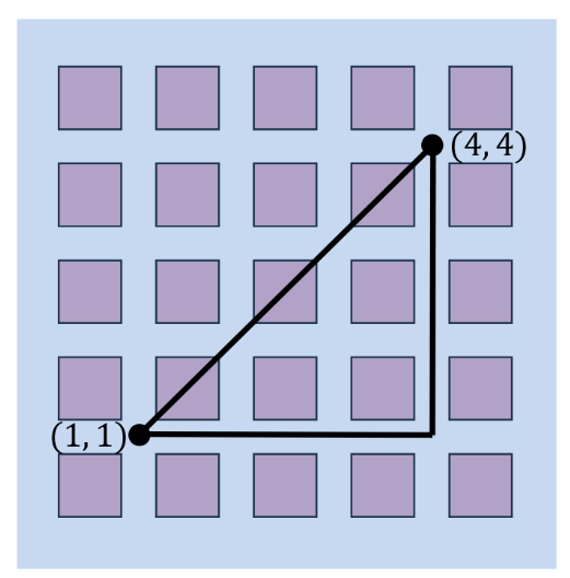
Euclidean
distance
Manhattan
distance
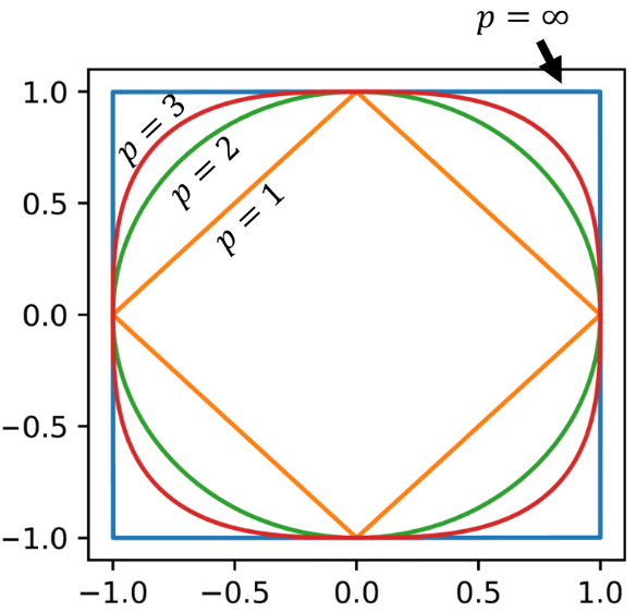
Behavior of \(p\)-Norms
-
The \(L^\infty\)-norm converges to the maximum entry of \(\mathbf{v}\)
-
The \(L^0\) "norm" provides the number of non-zero elements
this is a bit of a hack (hence "norm") by defining \(0^0=0\)
David Mayerich
STIM Laboratory, University of Houston
This graph shows the isovalue where \(||\mathbf{v}||_p = 1\) for \(\mathbf{v}\in \mathbb{R}^{2}\)
v_1
v_2
Properties of Matrix and Vector Norms
-
A matrix norm \(||\mathbf{A}||\) is induced by its vector norm \(||\mathbf{x}||\) such that they obey the following properties for \(\mathbf{x}\in \mathbb{C}^n\), \(\mathbf{A}\in \mathbb{C}^{n\times n}\), and \(\alpha \in \mathbb{C}\):
David Mayerich
STIM Laboratory, University of Houston
||\mathbf{A}||>0
\quad
\text{if}
\quad
\mathbf{A}\neq\mathbf{0}
||\alpha\mathbf{A}||=|\alpha|\ ||\mathbf{A}||
||\mathbf{A}+\mathbf{B}|| \leq ||\mathbf{A}|| + ||\mathbf{B}||
||\mathbf{I}||=1
||\mathbf{A}\mathbf{x}||
\leq
||\mathbf{A}||\ ||\mathbf{x}||
||\mathbf{A} \mathbf{B}|| \leq
||\mathbf{A}||\ ||\mathbf{B}||
Matrix Induced by \(L^p\)-Norms
David Mayerich
STIM Laboratory, University of Houston
||\mathbf{A}||_1=\max_{1\leq j \leq n}
\sum_{i=1}^n
|a_{ij}|
||\mathbf{A}||_\infty=\max_{1\leq i \leq n}
\sum_{j=1}^n
|a_{ij}|
sum the magnitude of all values in each column, taking the largest as the norm
sum the magnitude of all values in each row, taking the largest as the norm
||\mathbf{A}||_2=\sqrt{\lambda_0}
square root of the largest eigenvalue of \(\mathbf{A}\)
- The \(L^2\) norm is the most common, because it provides the tightest bound.
- Requires calculating the eigendecomposition of \(\mathbf{A}\)
- Can be approximated: \(||\mathbf{A}||_2 \leq \sqrt{||\mathbf{A}||_1 ||\mathbf{A}||_\infty}\)
Matrix Conditioning
Ill-Conditioned Systems
Condition Number
David Mayerich
STIM Laboratory, University of Houston
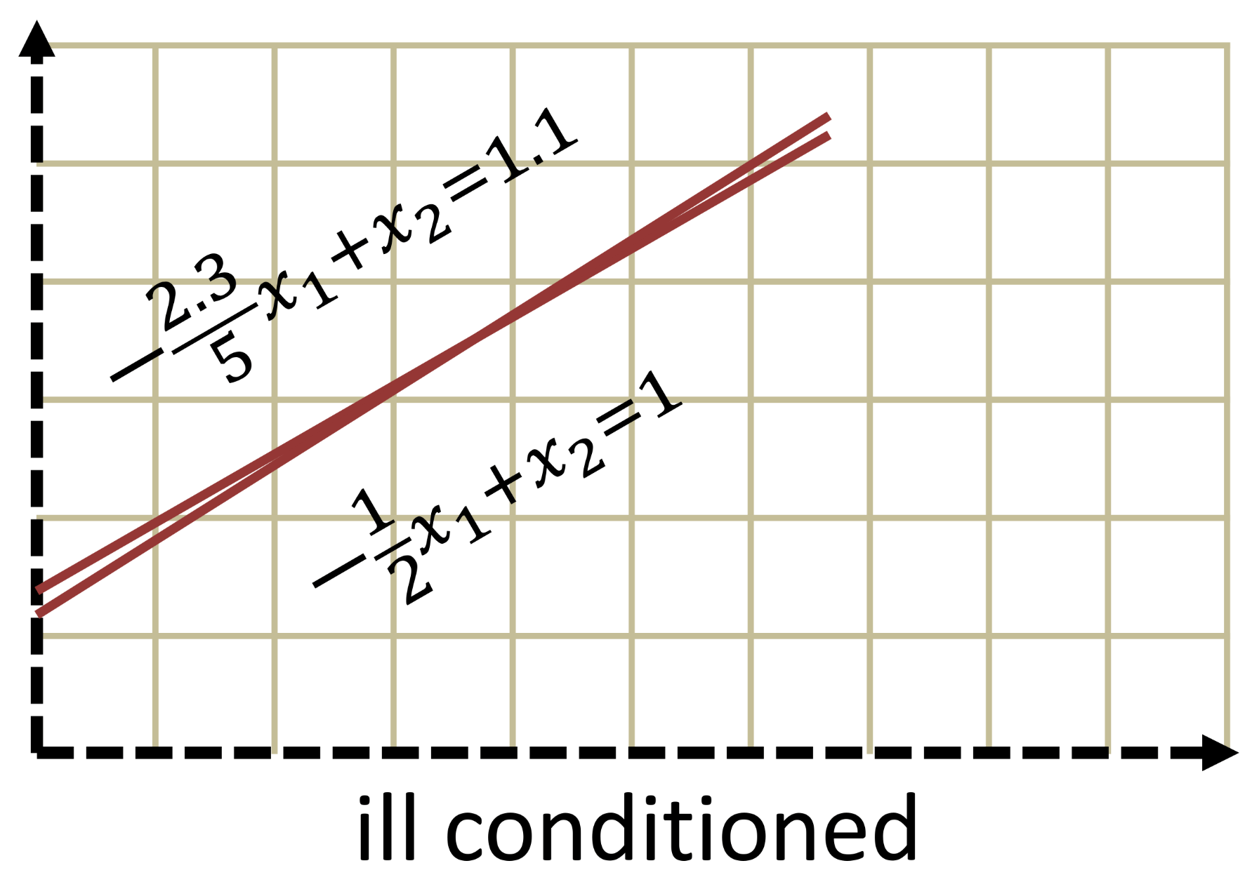
Ill-Conditioned Systems
-
Linear equations representing parallel planes do not have a single solution
-
Matrices representing these systems are singular (non-invertible)
-
Singular matrices have a determinant of zero: \(|\mathbf{A}|=0\)
-
Linear systems with planes that almost overlap are ill-conditioned
-
Ill-conditioned systems are sensitive to small changes in the right-hand-side
David Mayerich
STIM Laboratory, University of Houston
Does a small determinant suggest an ill-conditioned system?
\text{det}(\epsilon \mathbf{I})=\epsilon^n
Unfortunately no:
Examples of Ill-Conditioned Systems
David Mayerich
STIM Laboratory, University of Houston
\begin{bmatrix}
1 & 10 & 2- & 30 & 40 & 50\\
0 & 1 & 10 & 20 & 30 & 40\\
0 & 0 & 1 & 10 & 20 & 30\\
0 & 0 & 0 & 1 & 10 & 20\\
0 & 0 & 0 & 0 & 1 & 10\\
0 & 0 & 0 & 0 & 0 & 1
\end{bmatrix}
\mathbf{x}
=
\begin{bmatrix}
1510\\
1010\\
610\\
310\\
110\\
10
\end{bmatrix}
\begin{bmatrix}
1 & 10 & 2- & 30 & 40 & 50\\
0 & 1 & 10 & 20 & 30 & 40\\
0 & 0 & 1 & 10 & 20 & 30\\
0 & 0 & 0 & 1 & 10 & 20\\
0 & 0 & 0 & 0 & 1 & 10\\
0 & 0 & 0 & 0 & 0 & 1
\end{bmatrix}
\mathbf{x}
=
\begin{bmatrix}
1510\\
1010\\
610\\
310\\
110\\
10.001
\end{bmatrix}
\mathbf{x}=\begin{bmatrix}
10\\
10\\
10\\
10\\
10\\
10
\end{bmatrix}
\mathbf{x}=\begin{bmatrix}
-29.05\\
14.95\\
9.37\\
10.08\\
9.99\\
10.001
\end{bmatrix}
Matrix Condition Number
-
The sensitivity of the linear system to changes in right-hand-side values is quantified by the matrix condition number:
David Mayerich
STIM Laboratory, University of Houston
\kappa(\mathbf{A})=||\mathbf{A}||_2\ ||\mathbf{A}^{-1}||_2
-
A small condition number indicates that the system is relatively insensitive to input values (including roundoff errors)
-
A large condition number suggests that a system is highly sensitive and may not be solvable
What does the condition number show?
-
Given the linear system \(\mathbf{Ax}=\mathbf{b}\), assume a perturbation \(\mathbf{b}_\Delta\) in \(\mathbf{b}\) that results in a change \(\mathbf{x}_\Delta\) in the solution:
David Mayerich
STIM Laboratory, University of Houston
\mathbf{A}(\mathbf{x} + \mathbf{x}_\Delta)=\mathbf{b}+\mathbf{b}_\Delta
-
We want to describe \(\mathbf{x}_\Delta\) in terms of \(\mathbf{b}_\Delta\)
\mathbf{A}\mathbf{x} + \mathbf{A}\mathbf{x}_\Delta=\mathbf{b}+\mathbf{b}_\Delta
\mathbf{A}\mathbf{x}=\mathbf{b}
\mathbf{A}\mathbf{x}_\Delta=\mathbf{b}_\Delta
||\mathbf{A}||\ ||\mathbf{x}||\geq ||\mathbf{b}||
||\mathbf{x}||\geq \frac{||\mathbf{b}||}{||\mathbf{A}||}
\frac{1}{||\mathbf{x}||}\leq \frac{||\mathbf{A}||}{||\mathbf{b}||}
\mathbf{x}_\Delta=\mathbf{A}^{-1}\mathbf{b}_\Delta
||\mathbf{x}_\Delta||\leq||\mathbf{A}^{-1}||\ ||\mathbf{b}_\Delta||
\left(
\frac{1}{||\mathbf{x}||}
\right)
||\mathbf{x}_\Delta||\leq
\left(
\frac{||\mathbf{A}||}{||\mathbf{b}||}
\right)
||\mathbf{A}^{-1}||\ ||\mathbf{b}_\Delta||
since \(\frac{1}{||\mathbf{x}||}\leq \frac{||\mathbf{A}||}{||\mathbf{b}||}\), multiplying doesn't change the inequality
\frac{||\mathbf{x}_\Delta||}{||\mathbf{x}||}
\leq
\kappa(\mathbf{A})
\frac{||\mathbf{b}_\Delta||}{||\mathbf{b}||}
Conditioning and Precision Loss
-
If \(\kappa(\mathbf{A})=10^k\) then we expect to lose \(k\) digits of precision
-
If we know the coefficients of \(\mathbf{A}\) to \(t\)-digit precision, and \(\kappa(\mathbf{A}) \approx 10^k\), then the result is accurate to \(\approx 10^{t-k}\) digits
-
A similar analysis can be done for bits: if \(\kappa(\mathbf{A})=2^b\) then we expect to lose \(b\) bits of precision
-
The \(L^2\) norm is used in the definition of \(\kappa\), however this can be approximated using \(||\mathbf{A}||_2 \leq \sqrt{||\mathbf{A}_1||_1\ ||\mathbf{A}||_\infty}\)
David Mayerich
STIM Laboratory, University of Houston
E.3 Matrix Properties
By STIM Laboratory


