Interpolation
Numerical Methods
David Mayerich
Scalable Tissue Imaging and Modeling (STIM) Laboratory
Department of Electrical and Computer Engineering
Cullen College of Engineering
University of Houston
David Mayerich
STIM Laboratory, University of Houston

Specifying Functions
-
Formulaic or algorithmic:
David Mayerich
STIM Laboratory, University of Houston
f(x, y, n) = \cos(e^x) + \sin(y)j_n(x)
double f(double x, double y, int n) {
	return cos(exp(x)) + sin(y) * jn(n, x);
}
x, y, f \in \mathbb{R}
\quad
n \in \mathbb{N}
-
Look-up tables:
X \in \mathbb{R}^n = \{x_1, x_2, x_3, \cdots, x_n\}
F \in \mathbb{R}^n = \{f_1, f_2, f_3, \cdots, f_n\}
f(x_k)=F[k] = f_k
It is common to use a uniform spacing between samples: \(x_{n+1} = x_n + x_\Delta\)
double* cos_lut(int n) {
	double* lut = new double[n];
    double dx = (2.0 * M_PI) / (double)n;
    for(int i = 0; i < n; i++) {
        double x = i * dx;
        lut[i] = cos(x);
    }
    return lut;
}

int N = 100;
double theta = 1.23;
double* cos = cos_lut(N);
int xi = theta / (2 * M_PI) * N;
double cos_x = cos[xi];
Interpolation
-
Given a set of dependent variables \(X \in \mathbb{R}^N\) and corresponding function values \(F\in\mathbb{C}^N\), approximate \(f(x)\) where \(x\not\in X\)
-
Build a polynomial \(p(x)\) for all \(x\in\mathbb{R}\) such that:
David Mayerich
STIM Laboratory, University of Houston
\(X=[x_1, x_2, \cdots, x_N]\)
\(F=[f_1, f_2, \cdots, f_N]\)
\(p(x_i)=f_i\) for all \(N\) pairs \((x_i, f_i)\)
\(p(x_i)\) is said to interpolate the \((x_i, f_i)\) pairs
Polynomial Interpolation
-
Consider the case \(N=1\): \(X=[x_0]\) and \(F=[f_0]\)
-
A degree-0 polynomial can be defined to interpolation \(X\) and \(F\):
David Mayerich
STIM Laboratory, University of Houston
p(x)=f_1
-
Consider the case \(N=2\): \(X=[x_0, x_1]\) and \(F=[f_0, f_1]\)
-
A degree-1 polynomial (line) can interpolate \(X\) and \(F\):
p(x)= \left( \frac{x - x_1}{x_0 - x_1} \right)f_0 + \left( \frac{x-x_0}{x_1 - x_0} \right)f_1
= f_0 + \left( \frac{f_1-f_0}{x_1 - x_0} \right)\left( x-x_0 \right)
p_0(x)
p_1(x)
f_1
x_1
f_0
x_0
x_0
f_0
Lagrange Polynomials
-
We wish to interpolate an arbitrary set of \(N\) nodes
-
Select a set of cardinal polynomials \(L_0, L_1, \cdots, L_{N-1}\) such that:
David Mayerich
STIM Laboratory, University of Houston
L_i(x_j) =
\begin{cases}
0 & \text{ if } i \neq j\\
1 & \text{ if } i = j
\end{cases}
-
The interpolating polynomial can then be specified by:
p(x) = \sum_{i=1}^N L_i(x)f_i
-
Lagrange polynomials are suitable:
-
\(x\) is only in the numerator, so \(L_i\) is a degree-\((N-1)\) polynomial
-
What happens when \(x=x_i\)?
-
What happens when \(x=x_j\), when \(j\neq i\)?
-
L_i(x) =
\prod_{j=0, j\neq i}^{N-1}
\left(
\frac{x-x_j}{x_i - x_j}
\right)
Lagrange Polynomials
-
Plots of \(L_0\) through \(L_4\)
David Mayerich
STIM Laboratory, University of Houston
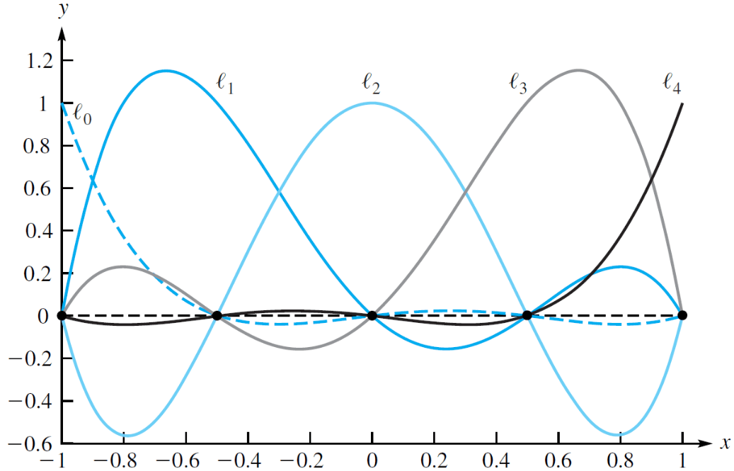
| x | y |
|---|---|
| -1.0 | 1.0 |
| -0.5 | 1.0 |
| 0.0 | 1.0 |
| 0.5 | 1.0 |
| 1.0 | 1.0 |
Polynomial Interpolation Theorem
-
An interpolating polynomial exists for any set of nodes and values
-
Theorem on the existence of polynomial interpolation:
David Mayerich
STIM Laboratory, University of Houston
If points \(x_0,x_1\cdots,x_{N-1}\) are distinct, there is a unique polynomial \(p(x)\) of degree at most \(N-1\) such that \(p(x_i)=f_i\) for \(0\leq i \leq N\) and arbitrary real values \(f_0, f_1\cdots, f_{N-1}\)
Uniqueness of the solution
-
Suppose that \(q(x)\) provides another interpolation of \(X\) and \(F\)
\(q(x_i)=f_i\) for \(0\leq i< N\) is of degree at most \(N-1\)
-
Then \(r(x)=q(x) - p(x)\) has the following properties:
-
degree of at most \(N-1\)
-
roots at the nodes \(X\)
-
-
Since any degree-\((N-1)\) polynomial has at most \(N-1\) roots, then \(q(x) = p(x)\)
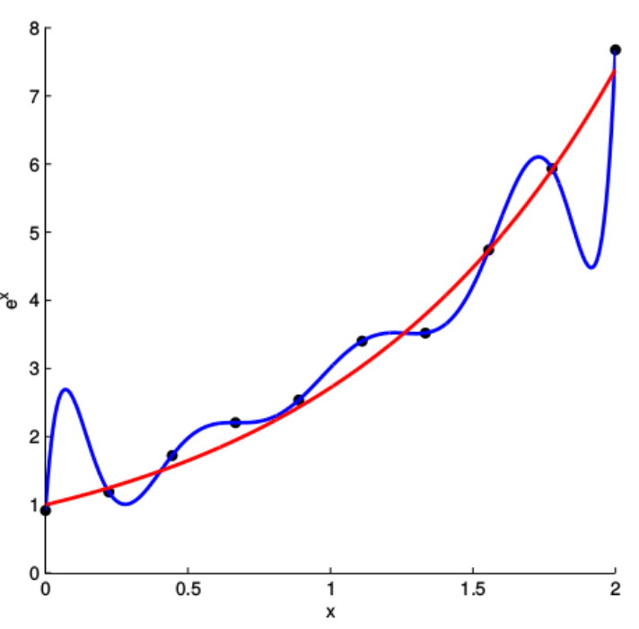
Problems with Polynomials
-
Measurements are inexact, often due to noise
-
Assume measurements of a function \(f(x)=e^x\) with 10 nodes and SNR=\(15\)dB
-
Interpolating polynomials tend to "wiggle"
David Mayerich
STIM Laboratory, University of Houston
Piecewise Interpolation
-
Use low-order methods that interpolate pieces of the data
David Mayerich
STIM Laboratory, University of Houston
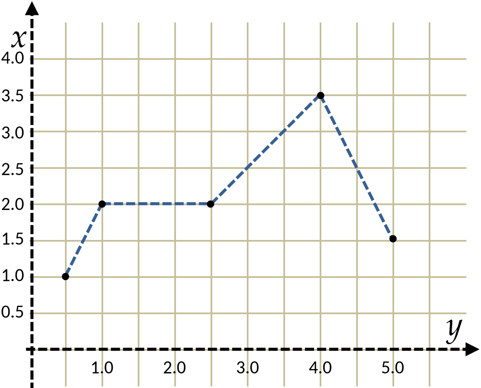
| x | y |
|---|---|
| 0.5 | 1.0 |
| 1.0 | 2.0 |
| 2.5 | 2.0 |
| 4.0 | 3.5 |
| 5.0 | 1.5 |
Advantages to Piecewise Interpolation
-
Linear interpolation between \(a=(x_0,f_0)\) and \(b=(x_1,f_1)\) is based on the Taylor series expansion:
David Mayerich
STIM Laboratory, University of Houston
p(a+x_\Delta)=p(a)+ p'(a)(x-a) + O\left(x_\Delta^2\right)
where \(p'(a)\approx \frac{p(b)-p(a)}{b-a}\)
-
This yields the \(L_1\) Lagrange polynomial:
L_1 = p(x)=f_0+ \frac{f_1 - f_0}{x_1 - x_0}(x - x_0)
-
Since this yields a consistent error term of \(O(x_\Delta^2)\), where \(x_\Delta\) is the distance between \(x\) and the nearest node \(x_0\) or \(x_1\)
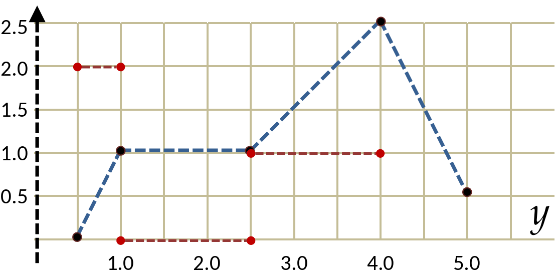
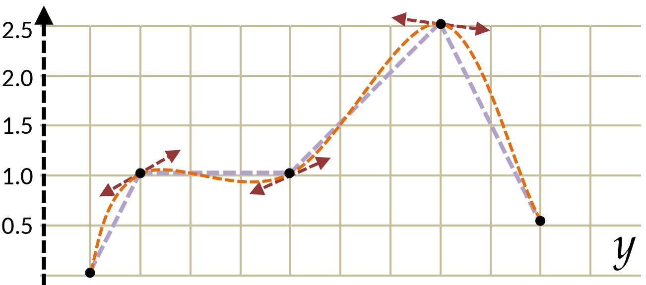
Differentiability Class
-
Classify piecewise interpolation based on the properties at nodes
-
An interpolated function \(f(x)\) is said to have differentiability class \(C^k\) if the first \(k\) derivatives \(f^{(1)}(x), f^{(2)}(x), \cdots, f^{(k)}(x)\) are continuous
-
"\(f(x)\) is \(C^2\) (\(C\)-two) continuous"
-
\(C^{\infty}\) functions are usually called "smooth"
-
-
What is the differentiability class of \(f(x)=|x|\)?
-
Linear interpolation:
David Mayerich
STIM Laboratory, University of Houston
Higher-Order Interpolation
-
Hermite interpolation: forces \(n\) derivatives to be continuous at nodes
-
Bezier curves: Use Bernstein polynomials as basis functions
-
These curves are usually piecewise and constrained to \(C^1\) at nodes:
David Mayerich
STIM Laboratory, University of Houston
F.1 Interpolation
By STIM Laboratory


