Lecture 3:
Tabular Reinforcement Learning
Artyom Sorokin | 19 Feb
Previous Lecture: Value Functions
Reward-to-go / Return:
G_t \doteq r(s_t, a_t) + \gamma r(s_{t+1}, a_{t+1}) + \gamma^2 r(s_{t+2}, a_{t+2}) + ...\, = \sum^{\infty}_{i=0} \gamma^{i} r(s_{t+i}, a_{t+i})
= \sum^{\infty}_{i=0} \gamma^i r_{t+i}
V_{\pi}(s) \doteq \mathbb{E}_{\pi} [ G_t| s_t = s] = \mathbb{E}_{\pi} \big[ \sum^{\infty}_{i=0} \gamma^i r_{t+i} | s_t = s \big]
Q_{\pi}(s, a) \doteq \mathbb{E}_{\pi} [ G_t| s_t = s, a_t = a] = \mathbb{E}_{\pi} \big[ \sum^{\infty}_{i=0} \gamma^i r_{t+i} | s_t = s, a_t = a \big]
State Value Function / V-Function:
State-Action Value Function / Q-Function:
Previous Lecture: Bellman Equations
Bellman Expectation Equations for policy \(\pi\):
V_{\pi}(s) = \sum_a \pi(a|s) \sum_{s^{\prime}} p(s'|s, a) [r + \gamma V_{\pi}(s^{\prime})]
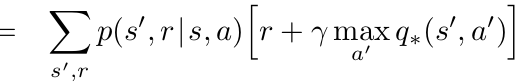
V_{*}(s) = max_{a} \sum_{s^{\prime}} p(s'|s, a) [r + \gamma V_{*}(s^{\prime})] = max_{a}\, Q_{*}(s,a)
Q_{\pi}(s, a) = \sum_{s^{\prime}} p(s'|s, a) [r + \gamma \sum_{a'} \pi(a'|s') Q_{\pi}(s', a')]
Q_{*}(s, a) = \sum_{s^{\prime}} p(s'|s, a) [r + \gamma \max_{a'} Q_{*}(s', a')]
Bellman Optimality Equations:
Previous Lecture: Bellman Equations
Bellman Expectation Equations for policy \(\pi\):
Bellman Optimality Equations:
Previous Lecture: Policy Iteration
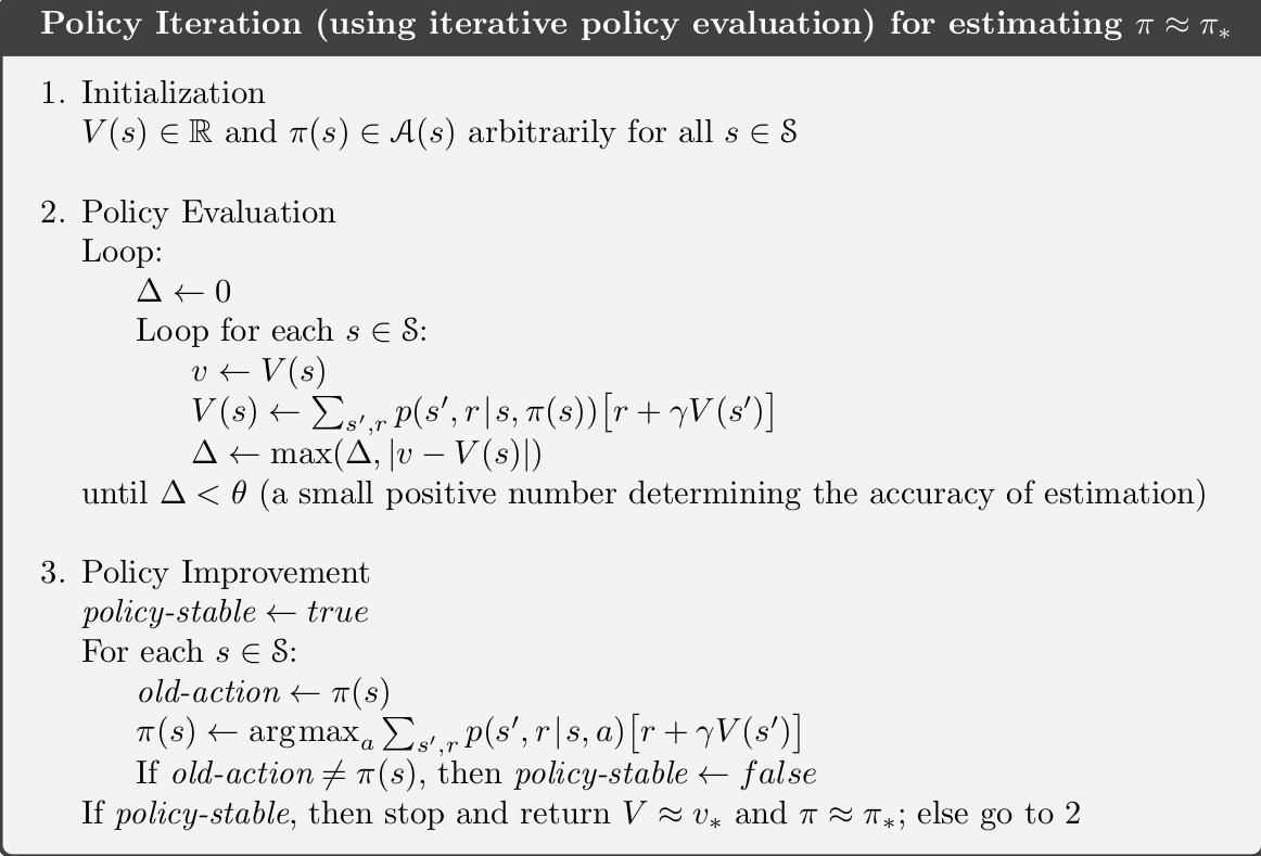
Use Belman Expectation Equations to learn \(V\)/\(Q\) for current policy
Greedily Update policy w.r.t. V/Q-function
Previous Lecture: Policy Iteration
Policy Evaluation steps
Policy Improvement steps
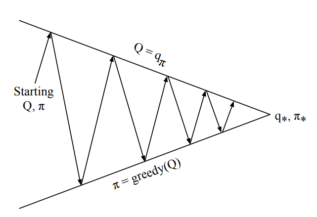
Generalized Policy Iteration
Imporves value function estimate for current policy \(\pi\)
Imporves policy \(\pi\)
w.r.t current value function
Previous Lecture: Value Iteration
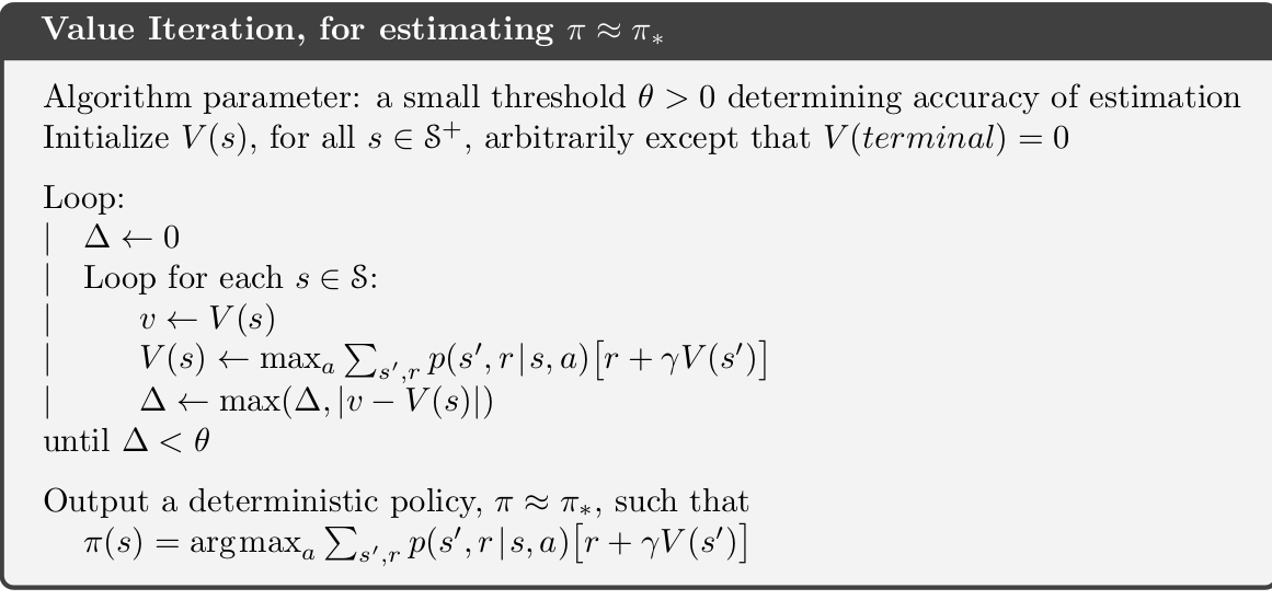
Use Belman Optimality Equations to learn \(V\)/\(Q\) for current policy
Policy Improvement is implicitly used here
But we don't know the model
V_{\pi}(s) = \sum_a \pi(a|s) \sum_{s^{\prime}} p(s'|s, a) [r + \gamma V_{\pi}(s^{\prime})]
Q_{\pi}(s, a) = \sum_{s^{\prime}} p(s'|s, a) [r + \gamma \sum_{a'} \pi(a'|s') Q_{\pi}(s', a')]
Solution: Use Sampling
- The model of the environment is unknown! :(
- But you still can interact with it!
Monte-Carlo Methods
GOAL: Learn value functions \(Q_{\pi}\) or \(V_{\pi}\) without knowing \(p(s'|s,a)\) and \(R(s,a)\)
RECALL that value function is the expected return:
Q_{\pi}(s,a) = \mathbb{E}_{\pi} [\sum^{\infty}_{k=0} \gamma^{k} r_{t+k+1}|S_t=s, A_t=a ]
First Visit Monte-Carlo
By Law of Large Numbers, \(q(s,a) \rightarrow Q_{\pi}(s,a)\) as \(N(s,a) \rightarrow \infty\)
IDEA: Estimate expectation \(Q_{\pi}(s,a)\) with empirical mean \(q(s,a)\):
- Generate an episode with \(\pi\)
- The first time-step \(t\) that state-action \((s,a)\) is visited
- Increment counter \(N(s,a) = N(s,a) + 1\)
- Increment total return \(S(s,a) = S(s,a) + G_t\)
- Value is estimated by mean return \(q(s,a) = S(s,a)/N(s,a)\)
Monte-Carlo Methods: Prediction
We can update mean values incrementally:
Incremental Monte Carlo Update:
\mu_{k+1} = \frac{1}{k+1} \sum^{k+1}_{i=1} x_i = \mu_{k} + \frac{1}{k+1} (x_{k+1} - \mu_{k})
Prediction error
Old estimate
Learning rate
q(s_t,a_t) \leftarrow q(s_t, a_t) + \frac{1}{N(s_t,a_t)} (G_t - q(s_t,a_t))
In non-stationary problems we can fix learning rate:
q(s_t,a_t) \leftarrow q(s_t,a_t) + \alpha (G_t - q(s_t,a_t))
Monte-Carlo Methods
- MC methods learn directly from episodes of experience
- MC is model-free: no knowledge of MDP transitions / rewards
- MC learns from complete episodes: no bootstrapping
- MC uses the simplest possible idea: value = mean return
- Caveat: can only apply MC to episodic MDPs:
- All episodes must terminate
Monte-Carlo Methods: Control
Remember Policy Iteration?
How would look PI version with Monte-Carlo Policy Evaluation?
Questions:
- Why we estimate \(Q_{\pi}\) and not \(V_{\pi}\)?
- Do you see any problem with policy improvement step?

- Policy Evaluation: Monte-Carlo Evaluation, \(q = Q_{\pi}\)
- Policy Improvement: Greedy policy improvement, i.e. \(\pi'(s) = argmax_a q(s,a)\)
Eploration-Exploitation Problem
Agent can't visit every \((s,a)\) with greedy policy!
Agent can't get correct \(q(s,a)\) estimates without visiting \((s,a)\) frequently!
(i.e. remember law of large numbers)

Monte-Carlo Methods: Control
Use \(\epsilon\)-greedy policy:
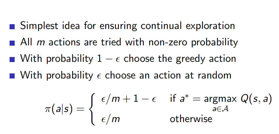
- Simplest idea for ensuring continual exploration
- All \(m\) actions are tried with non-zero probability
- With probability \(1 − \epsilon\) choose the greedy action
- With probability \(\epsilon\) choose an action at random
Monte-Carlo Methods: Control
Monte-Carlo Method
Policy Iteration with Monte-Carlo method:
For every episode:
- Policy Evaluation: Monte-Carlo Evaluation, \(q = Q_{\pi}\)
- Policy Improvement: \(\epsilon\)-greedy policy improvement
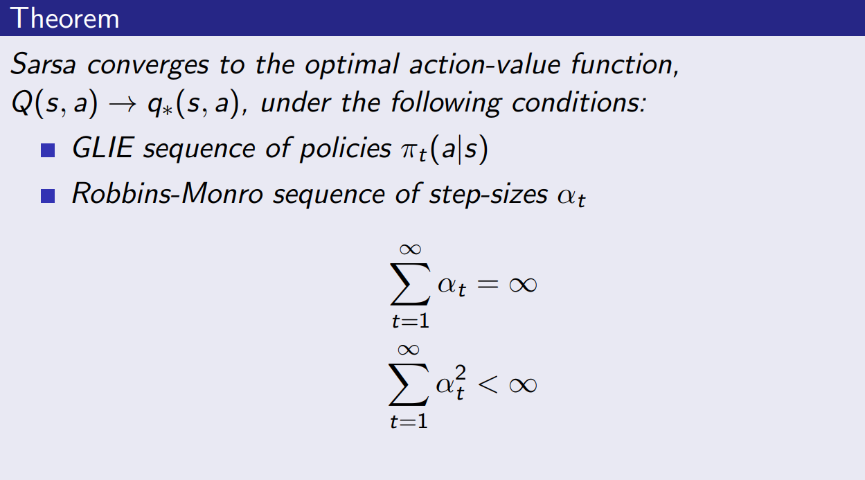
Monte-Carlo Methods: GLIE
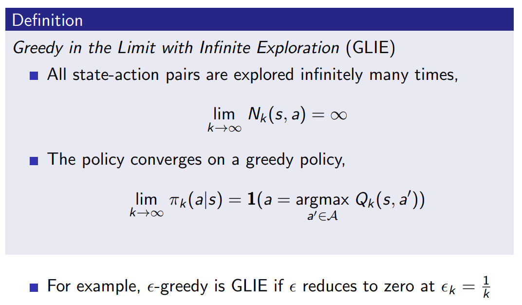
Monte-Carlo Methods: GLIE
GLIE Mont-Carlo Control:
- Sample k-th episode using curent policy \(\pi\)
- Update with \(q(s,a)\) with \(1/N(s,a)\) learning rate
- Set \(\epsilon = 1/k\)
- Use \(\epsilon\)-greedy policy improvement
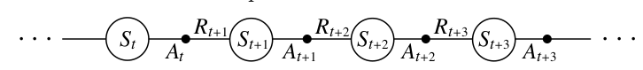
Temporal Difference Learning
Problems with Monte-Carlo method:
- Updates policy only once per episode, i.e. only episodic MDPs
- Doesn't use MDP properties
Solution:
- Recall Bellman equation:
- Use sampling instead of knowledge about the model:
Q_{\pi}(s, a) = \sum_{s^{\prime}} p(s'|s, a) [r + \gamma \sum_{a'} \pi(a'|s') Q_{\pi}(s', a')]
q_{\pi}(s, a) = \textcolor{blue}{\mathbb{E}_{s'}} [r + \gamma \textcolor{blue}{\mathbb{E}_{a'}}\,q_{\pi}(s', a')] =
\textcolor{blue}{\mathbb{E}_{\tau}}[r + \gamma q_{\pi}(s', a')]
TD-learning: Prediction
Goal: learn \(Q_{\pi}\) online from experience
Incremental Monte-Carlo:
- Update value \(q(s_t, a_t)\) toward actual return \(G_t\)
Temporal-Difference learning:
- Update value \(q(s_t, a_t)\) toward estimated return \(r_{t+1} + \gamma q(s_{t+1}, a_{t+1})\)
\(r_{t+1} + \gamma q(s_{t+1}, a_{t+1})\) is called the TD target
\(\delta_t = r_{t+1} + \gamma q(s_{t+1}, a_{t+1}) - q(s_t, a_t)\) is called the TD error
q(s_t,a_t) \leftarrow q(s_t,a_t) + \alpha (\textcolor{red}{G_t} - q(s_t,a_t))
q(s_t,a_t) \leftarrow q(s_t,a_t) + \alpha (\textcolor{red}{r_t + \gamma q(s_{t+1},a_{t+1})} - q(s_t,a_t))
Temporal Difference Learning
Temporal Difference Learning:
- TD methods learn directly from episodes of experience
- TD is model-free: no knowledge of MDP transitions / rewards
- TD learns from incomplete episodes, by bootstrapping
- TD updates a guess towards a guess
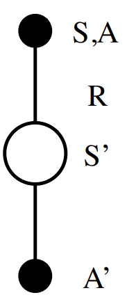
TD-learning: SARSA update
q(s_t,a_t) \leftarrow q(s_t,a_t) + \alpha (r_t + \gamma q(s_{t+1},a_{t+1}) - q(s_t,a_t))
This update is called SARSA: State, Action, Reward, next State, next Action
TD-learning: SARSA as Policy Iteration
Policy Iteration with Temporal Difference Learning:
For every step:
- Policy Evaluation: SARSA Evaluation, \(q = Q_{\pi}\)
- Policy Improvement: \(\epsilon\)-greedy policy improvement
TD-learning: SARSA algorithm
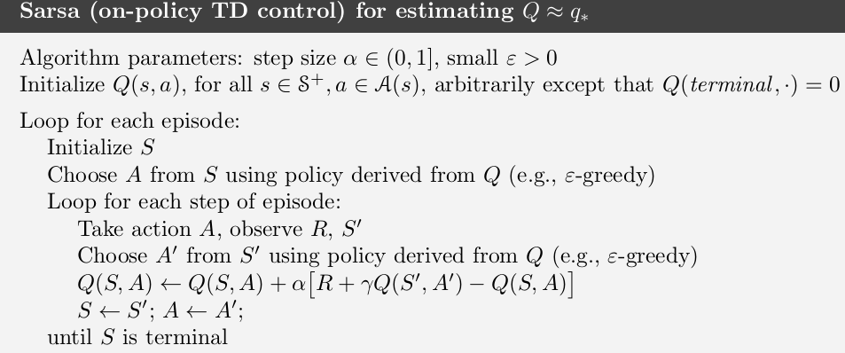
TD-learning: SARSA
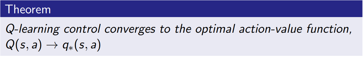
TD-learning: Q-Learning
We approximate Bellman Expectation Equation with SARSA update:
Can we utilize Bellman Optimality Equation for TD-Learning?
Q_{\pi}(s, a) = \sum_{s^{\prime}} p(s'|s, a) [r + \gamma \sum_{a'} \pi(a'|s') Q_{\pi}(s', a')]
Q_{*}(s, a) = \sum_{s^{\prime}} p(s'|s, a) [r + \gamma \max_{a'} Q_{*}(s', a')]
q(s, a) = \textcolor{blue}{\mathbb{E}_{s'}} [r + \gamma \max_{a'} q(s', a')]
Yes, of course:
TD-learning: Q-Learning vs SARSA
From Bellman Expectation Equation (SARSA) :
From Bellman Optimality Equation (Q-Learning):
q(s, a) = \textcolor{blue}{\mathbb{E}_{s'}} [r + \gamma \textcolor{blue}{\mathbb{E}_{a'}}\,q(s', a')]
q(s, a) = \textcolor{blue}{\mathbb{E}_{s'}} [r + \gamma \max_{a'} q(s', a')]
\(a'\) comes from the policy \(\pi\) that generated this experience!
No connection to the actual policy \(\pi\)
TD-learning: Q-Learning vs SARSA
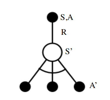
Q-Learning Update:
q(s_t,a_t) \leftarrow q(s_t,a_t) + \alpha (r_t + \gamma \textcolor{blue}{max_{a'}}\,q(s_{t+1},\textcolor{blue}{a'}) - q(s_t,a_t))
q(s_t,a_t) \leftarrow q(s_t,a_t) + \alpha (r_t + \gamma q(s_{t+1},a_{t+1}) - q(s_t,a_t))
SARSA Update:
TD-learning: Q-Learning
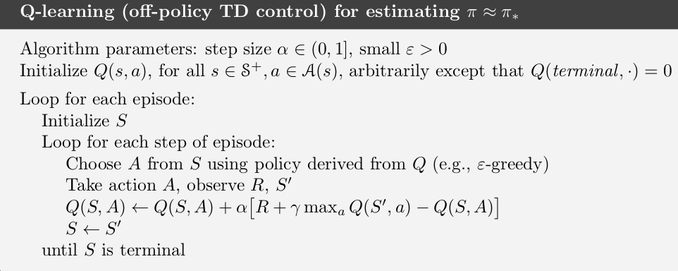
On-policy vs Off-Policy Algorithms
SARSA and Monte-Carlo are on-policy algorithms:
- Improve policy \(\pi_k\) only from experience sampled with this policy \(\pi_k\)
- Can't use old trajectories sampled with \(\pi_{k-i}\)
Q-Learning is off-policy algorithm:
- Can Learn policy \(\pi\) using experience generated with other policy \(\mu\)
- Learn from observing humans or other agents
- Re-use experience generated from old policies
- Learn about optimal policy while following exploratory policy
- Learn about multiple policies while following one policy
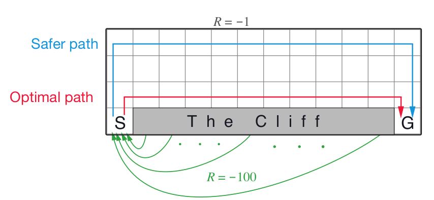
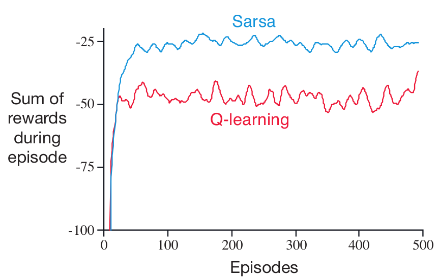
TD-learning: Cliff Example
TD vs MC: Driving Home Example
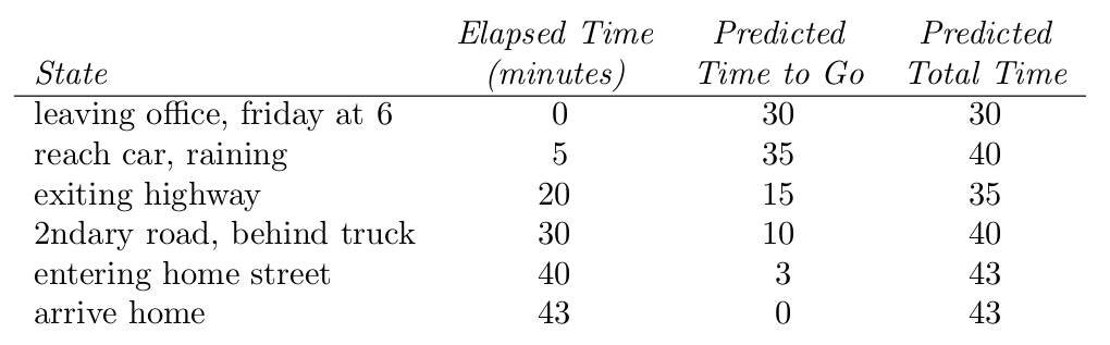
TD vs MC: Driving Home Example
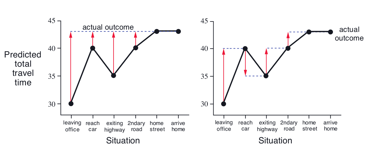
Monte Carlo
Temporal Difference
TD vs MC: Bias-Variance Tradeoff
- Return \(G_t = R_{t+1} + \gamma R_{t+2} + ... + \gamma^{T-t-1}R_{T}\) is unbiased estimate of \(Q_{\pi}(s_t, a_t)\)
- True TD target \( R_{t+1} + \gamma Q_{\pi}(s_{t+1},a_{t+1}) \) is unbiased estimate of \(Q_{\pi}(s_t, a_t)\)
- TD target \( R_{t+1} + \gamma q(s_{t+1},a_{t+1}) \) is biased estimate of \(Q_{\pi}(s_t, a_t)\)
- TD target has lower variance than the return:
- Return depends on many random actions, transitions, rewards
- TD target depends on one random action, transition, reward
- Monte-Carlo Methods: high variance, no bias
- TD-Обучение: low variance, has bias
TD vs MC: Bias-Variance Tradeoff
- MC has high variance, zero bias
- Good convergence properties
- (even with function approximation)
- Not very sensitive to initial value
- Very simple to understand and use
- TD has low variance, some bias
- Usually more efficient than MC
- TD converges to \(Q_{\pi}(s,a)\)
- (but not always with function approximation)
- More sensitive to initial value
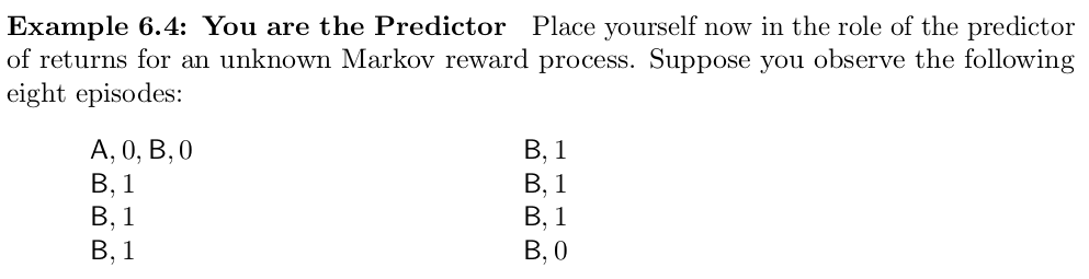
TD vs MC: AB Example
Monte-Carlo Backup
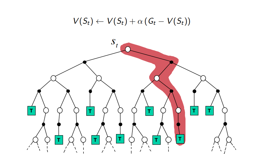
q(s_t,a_t) \leftarrow q(s_t,a_t) + \alpha (G_t - q(s_t,a_t))
Temporal-Difference Backup
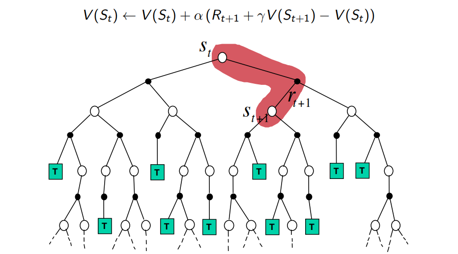
q(s_t,a_t) \leftarrow q(s_t,a_t) + \alpha (r_t + \gamma q(s_{t+1},a_{t+1}) - q(s_t,a_t))
Sampling and Bootstrapping
-
Bootstrapping: update involves an estimate
- MC does not bootstrap
- DP bootstraps
- TD bootstraps
-
Sampling: update samples an expectation
- MC samples
- DP does not sample
- TD samples
Sampling and Bootstrapping

N-step Returns
\textcolor{red}{n=1}\,\,\,\,\,\,\,\, G^{(1)}_t = R_{t+1} + \gamma Q(S_{t+1}, A_{t+1})
\textcolor{red}{n=2}\,\,\,\,\,\,\,\, G^{(2)}_t = R_{t+1} + \gamma R_{t+2} + \gamma^{2} Q(S_{t+2}, A_{t+2})
\textcolor{red}{n=\infty}\,\,\,\,\, G^{(\infty)}_t = R_{t+1} + \gamma R_{t+2} + ... + \gamma^{T-t-1} R_{T}
Consider the following n-step returns for n = 1, 2, ...:
n-step Temporal Difference Learning:
.
.
.
.
.
.
q(s_t,a_t) \leftarrow q(s_t,a_t) + \alpha (G^{(n)}_t - q(s_t,a_t))
(MC)
(TD: SARSA)
Combining N-step Returns
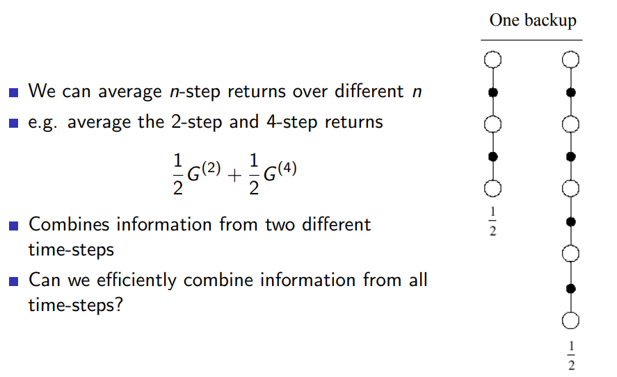
We can average n-step returns over different n,
e.g. average the 2-step and 4-step returns:
G^{(x)}_t = \frac{G^{(2)}_t + G^{(4)}_t}{2}
- Can we combine information from all n-step returns?
- Yes! Turns out that it is easier to use this combination than selecting right value of \(n\) for n-step return.
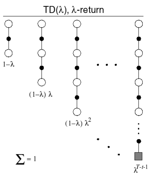
TD(\(\lambda\))
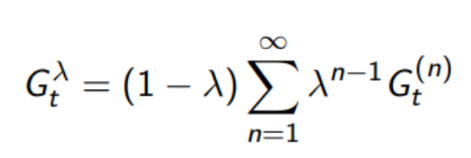
- The \(\lambda\)-return \(G^{\lambda}_t\) combines all n-step returns \(G^{(n)}_t\)
- Using weight \((1 −\lambda) \lambda^{n-1}\)
G^{\lambda}_t = (1 - \lambda) \sum^{\infty}_{n=1} \lambda^{n-1} G^{(N)}_{t}
- Forward-view TD(\(\lambda\))... actually SARSA(\(\lambda\)):
q(s_t,a_t) \leftarrow q(s_t,a_t) + \alpha (G^{\lambda}_t - q(s_t,a_t))
TD(0) and TD(1):
But why?
What happens when \(\lambda = 0\)?
G^{\lambda=0}_t = G^{1}_t = R_{t+1} + \gamma Q(S_{t+1}, A_{t+1})
i.e. TD target
What happens when \(\lambda = 1\)?
G^{\lambda=1}_t = G^{\infty}_t = R_{t+1} + \gamma R_{t+2} + ... + \gamma^{T-t-1} R_T
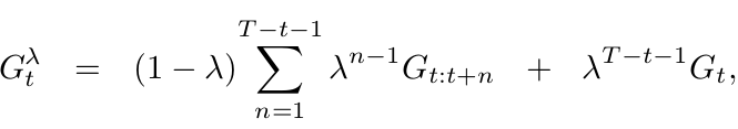
We can rewrite \(G^{\lambda}_t\) as:
i.e. MC target
G^{\lambda}_t =(1 - \lambda) \sum^{T-t-1}_{n=1} \lambda^{n-1} G^{(n)}_t + (1-\lambda) \sum^{\infty}_{n=T-t} \lambda^{n-1} G^{\infty}_{t}
G^{\lambda}_t =(1 - \lambda) \sum^{T-t-1}_{n=1} \lambda^{n-1} G^{(n)}_t + \lambda^{T-t-1} G^{\infty}_{t} \frac{(1-\lambda)}{(1-\lambda)}
TD(0) and TD(1):
What happens when \(\lambda = 0\)?
G^{\lambda=0}_t = G^{1}_t = R_{t+1} + \gamma V(S_{t+1})
i.e. just TD-learning
What happens when \(\lambda = 1\)?
G^{\lambda=1}_t = G^{\infty}_t = R_{t+1} + \gamma R_{t+2} + ... + \gamma^{T-t-1} R_T
i.e. Monte-Carlo learning
We can rewrite \(G^{\lambda}_t\) as:
HOW?
TD(\(\lambda\)): Forward view
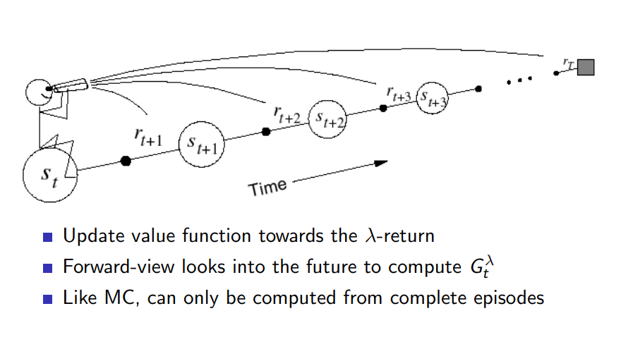
- Update value function towards the \(\lambda\)-return
- Forward-view looks into the future to compute \(G^{\lambda}_{t}\)
- Like MC, can only be computed from complete episodes
Text
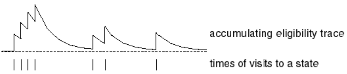
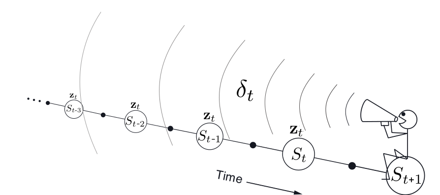
TD(\(\lambda\)): Backward View
- Credit assignment problem: did bell or light cause shock?
- Frequency heuristic: assign credit to most frequent states
- Recency heuristic: assign credit to most recent states
- Eligibility traces combine both heuristics
E_0(s,a) = 0
E_t(s,a) = \gamma \lambda E_{t-1}(s,a) + \mathbf{1}[S_t = s, A_t = a]

Eligibility Traces: SARSA(\(\lambda\))
- Keep an eligibility trace for every state \(s\)
- Update value \(q(s, a)\) for every (\(s, a\)) with non zero \(E_t(s,a)\)
- In proportion to TD-error \(\delta_t\) and eligibility trace \(E_t(s,a)\)
\delta_t = r_{t+1} + \gamma q(s_{t+1}, a_{t+1}) - q(s_t, a_t)
q(s,a) \leftarrow q(s,a) + \alpha \delta_t E_t(s,a)
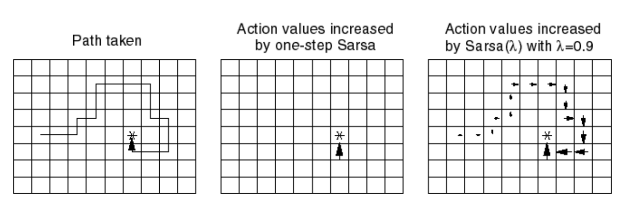
SARSA(\(\lambda\)) vs SARSA
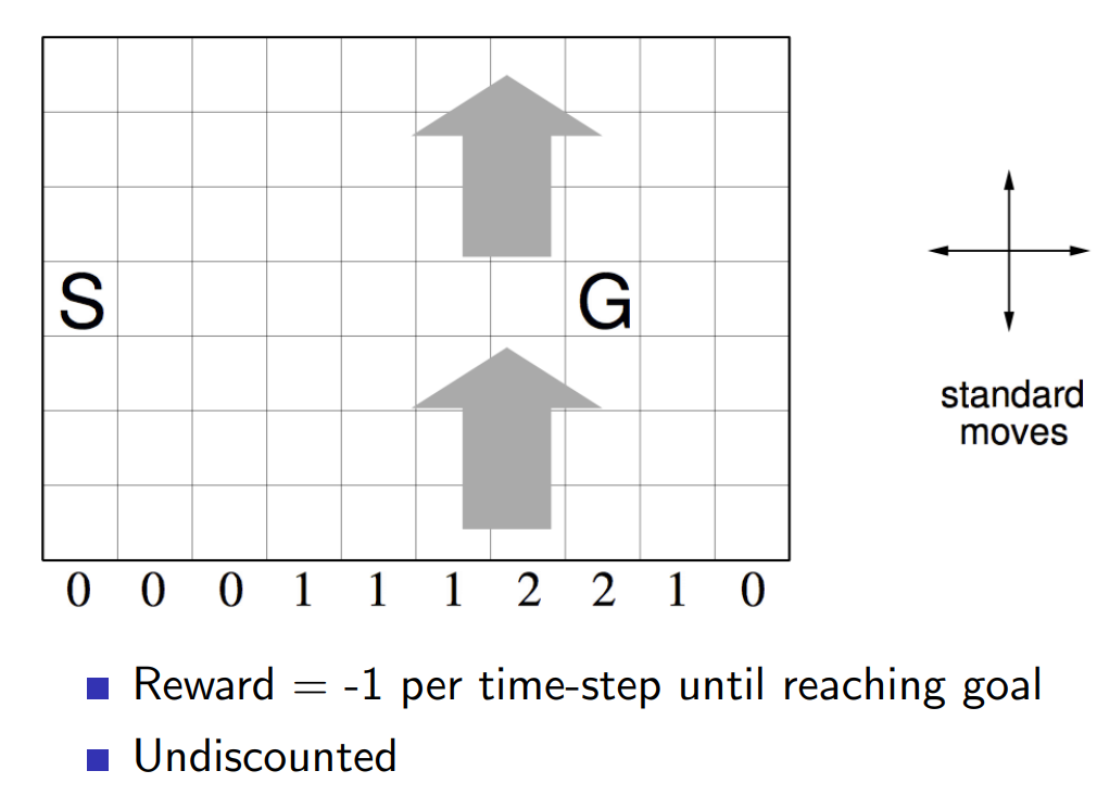
SARSA(\(\lambda\)) vs SARSA
Tabular RL: Resume
- Monte-Carlo and Temporal-Difference learning use sampling to approximate Dynamic Programming Methods
- TD learning assumes MDP and use bootstraping updates
Thank you for your attention!
03 - Tabular RL
By supergriver


