Lecture 12:
Exploration
Artyom Sorokin |4 May
What is the problem?
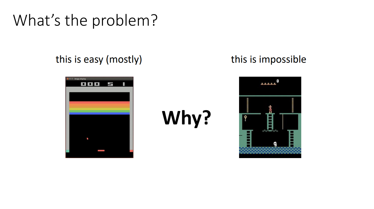
Monstezuma's Revenge

- Getting key = reward
- Opening door = reward
- Getting killed by skull = nothing (is it good? bad?)
- Finishing the game only weakly correlates with rewarding events
- We know what to do because we understand what these sprites mean!
To get the first reward:
go down the first ladder -> jump on the rope -> jump on the second ladder -> go down the second ladder -> avoid skull -> ...
Exploration and exploitation
-
Two potential definitions of exploration problem
- How can an agent discover high-reward strategies that require a temporally extended sequence of complex behaviors that, individually, are not rewarding?
- How can an agent decide whether to attempt new behaviors (to discover ones with higher reward) or continue to do the best thing it knows so far?
-
Actually the same problem:
- Exploitation: doing what you know will yield highest reward
- Exploration: doing things you haven’t done before, in the hopes of getting even higher reward
Exploration is Hard
Can we derive an optimal exploration strategy?
Yes (theoretically tractable)
No ( theoretically intractable)
multi-armed bandits
contextual bandits
small, finite MDPs
large, infinite MDPs
can formalize exploration as POMDP identification
optimal methods don’t work …but can take inspiration from optimal methods
Muliti-Armed Bandits: Reminder

Solving Exploration in Bandits
Bandit Example:
- assume \(r(a_i) \sim p_{\theta_i}(r_i)\),
- e.g. \(p(r_i=1) = \theta_i\) and \(p(r_i=0) = 1- \theta_i\)
- prior on \(\theta\) : \(\theta \sim p(\theta)\)
This defines a POMDP with states: \(s = [\theta_1, ..., \theta_n]\),
where belief states are \(\hat{p}(\theta_1,..., \theta_n)\)
- solving the POMDP yields the optimal exploration strategy
- but that’s overkill: belief state is huge!
- we can do very well with much simpler strategies
How to measure goodness of exploration algorithm?
Regret: difference between optimal policy and ours
Reg(T) = T \mathbb{E}[r(a^{*})] - \sum^{T}_{t=1} r(a_t)
How can we beat the bandit?
Reg(T) = T \mathbb{E}[r(a^{*})] - \sum^{T}_{t=1} r(a_t)
- Variety of relatively simple strategies
- Often can provide theoretical guarantees on regret
- Variety of optimal algorithms (up to a constant factor)
- But empirical performance may vary…
- Exploration strategies for more complex MDP domains will be inspired by these strategies
Optimimism in Face of Uncertainty
keep track of average reward \(\hat{\mu}_a\) for each action \(a\)
exploitation: pick \(a = argmax\,\hat{\mu}_a\)
optimistic estimate: \(a = argmax\,\hat{\mu}_a + C \sigma_a\)
Intuition: try each arm until you are sure it's not great
how uncertain we are about this action
Example:
a = argmax\,\hat{\mu}_a + \sqrt{\frac{2\,ln T}{N(a)}}
\(Reg(T)\) is \(O(log\,T)\) as good as possible
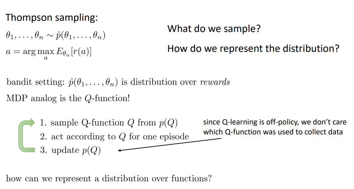
Posterior Sampling
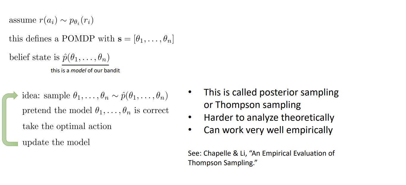
Bandit Example:
- assume \(r(a_i) \sim p_{\theta_i}(r_i)\),
- this defines a POMDP with states: \(s = [\theta_1, ..., \theta_n]\),
- belief states are \(\hat{p}(\theta_1,..., \theta_n)\)
- This is called posterior sampling or Thompson sampling
- Harder to analyze theoretically
- Can work very well empirically
Correction:
Thompson sampling is asymptotically optimal!
https://arxiv.org/abs/1209.3353
Information Gain
We want to determine some latent variable \(z\)
(e.g. optimal action, q-value, parameters of a model)
Which action do we take to determine \(z\) ?
let \( H(\hat{p}(z))\) be the current entropy of our \(z\) estimate
let \( H(\hat{p}(z)|y)\) be the entropy of our \(z\) estimate after observation \(y\)
Entropy measures lack of information.
IG(z;y) = \mathbb{E}_y[H(\hat{p}(z)) - H(\hat{p}(z)|y) ]
Then Information Gain measures how much information about \(z\) we can get by observing \(y\)
Information Gain Example
IG(z;y|a) = \mathbb{E}_y[H(\hat{p}(z)) - H(\hat{p}(z)|y)|a]
\(y=r_a\), \(z = \theta_a\) (parameters of a model)
\(g(a) = IG(\theta_a; r_a|a)\) - information gain for action \(a\)
\(\Delta(a) = E[r(a^*) - r(a)]\) - expected suboptimality of a
Policy: choose actions according to:
argmin_a\,\Delta(a)^2/ g(a)
General Ideas
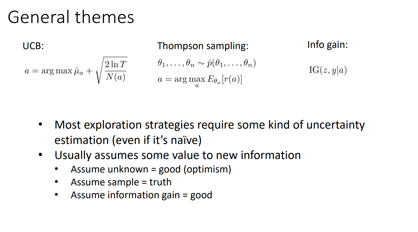
- Most exploration strategies require some kind of uncertainty estimation (even if it’s naïve)
- Usually assumes some value to new information
- Assume unknown = good (optimism)
- Assume sample = truth
- Assume information gain = good
UCB:
Thompson sampling:
Info Gain:
IG(z;y|a)
argmax\,\hat{\mu}_a + \sqrt{\frac{2\,ln T}{N(a)}}
Why Should We Care?
- Bandits are easier to analyze and understand
- Can derive foundations for exploration methods
- Then apply these methods to more complex MDPs
- Not covered here:
- Contextual bandits (bandits with state, essentially 1-step MDPs)
- Optimal exploration in small MDPs
- Bayesian model-based reinforcement learning (similar to information gain)
- Probably approximately correct (PAC) exploration
Exploration in Deep RL
-
Optimistic exploration / Curiocity:
- new state = good state
- requires estimating state visitation frequencies or novelty
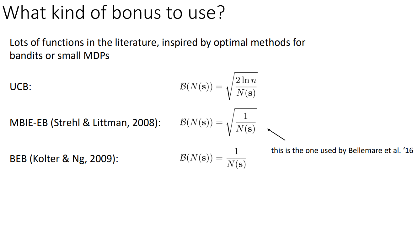
- typically realized by means of exploration bonuses
-
Thompson sampling style algorithms:
- learn distribution over Q-functions or policies
- sample and act according to sample
-
Information gain style algorithms:
- reason about information gain from visiting new states
Curiocity /Optimistic Exploration
Can we use this idea with MDPs?
a = argmax\,\hat{\mu}_a + \sqrt{\frac{2\,ln T}{\textcolor{black}{N(a)}}}
UCB:
Yes! Add exploration bonus (based on \(N(s,a)\) or \(N(s)\)) to the reward:
r^{+}(s,a) = r(s,a) + \mathbb{\Beta}(N(s,a))
This should work as long as \(\mathbf{B}(N(s,a))\) decrease with \(N(s,a)\)
Use \(r^{+}(s,a)\) with any model-free algorithm!
But the is one problem...
The Trouble with Counts
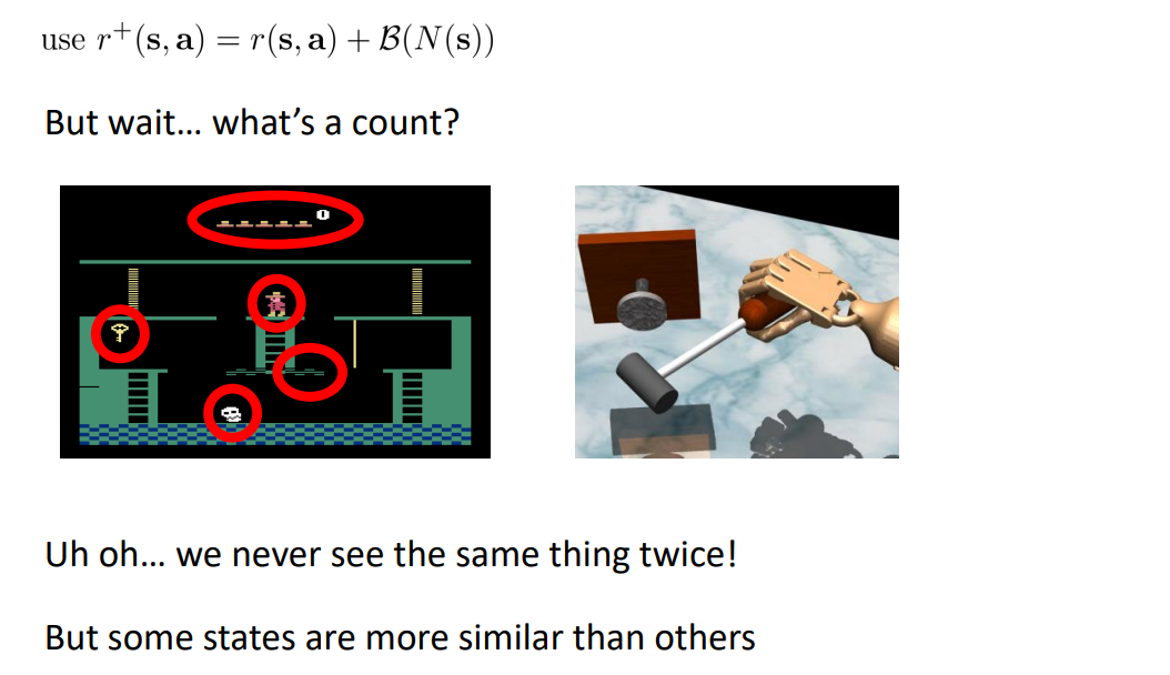
- We never see the same thing twice!
- But some states are more similar than others
r^{+}(s,a) = r(s,a) + \mathbb{\Beta}(\textcolor{red}{N(s,a)})
But wait… what’s a count?
Fitting Generative Models
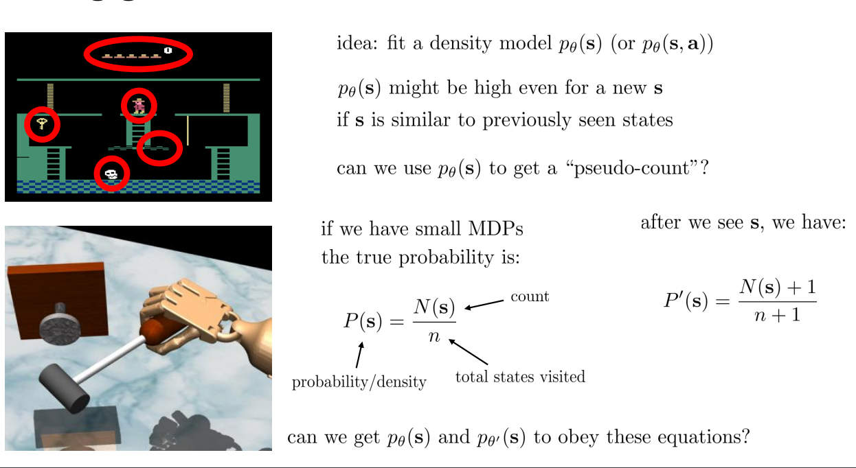
Idea: fit a density model \(p_{\theta}(s)\)
\(p_{\theta}(s)\) might be high even for a new \(s\) if \(s\) is similar to previously seen states.
Can we \(p_{\theta}(s)\) to get a "pseudo-count"?
The true probability is:
P(s) = \frac{N(s)}{n}
P'(s) = \frac{N(s)+1}{n+1}
After visiting \(s\):
GOAL:
To create \(p_{\theta}(s)\) and \(p_{\theta'}(s)\) that obey these equations!
Exploring with Pseudo-Counts
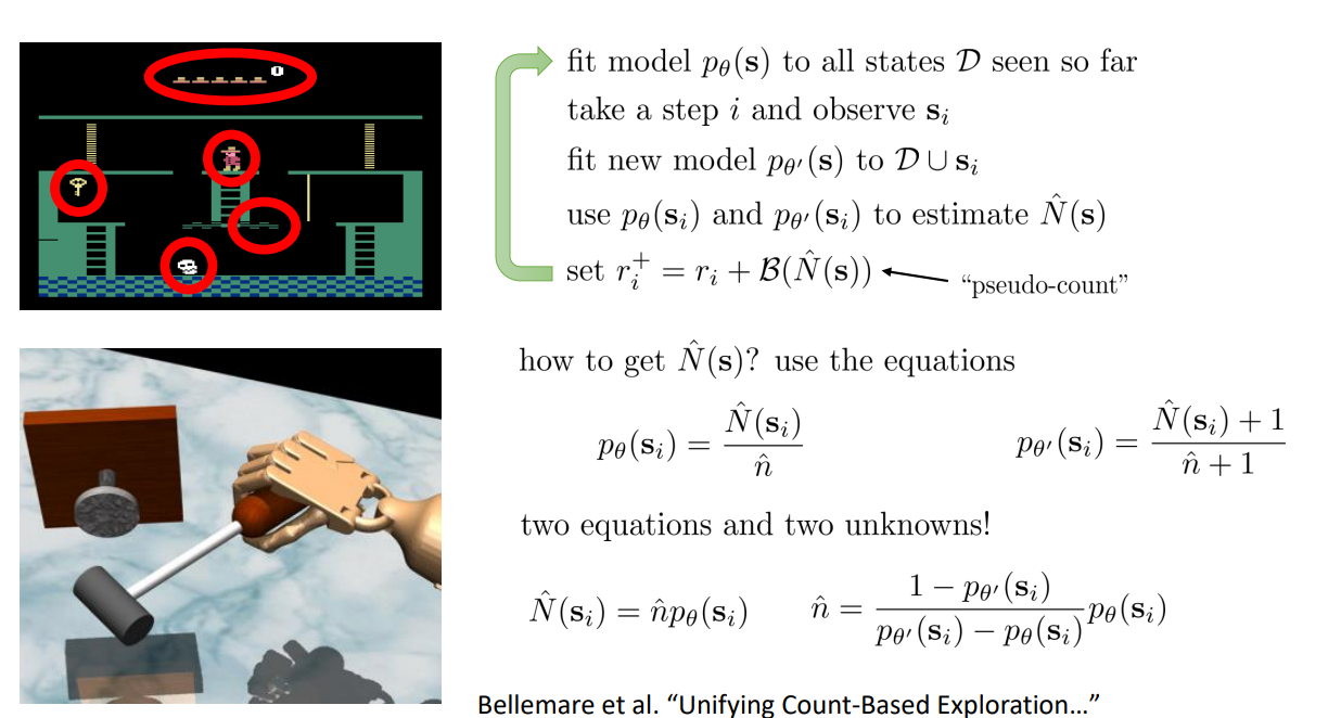
p_{\theta}(s) = \frac{\textcolor{red}{\hat{N}}(s)}{\textcolor{blue}{\hat{n}}}
Solve a system of two linear equations:
p_{\theta'}(s) = \frac{\textcolor{red}{\hat{N}}(s) + 1}{\textcolor{blue}{\hat{n}}+1}
GOAL:
To create \(p_{\theta}(s)\) and \(p_{\theta'}(s)\) that obey these equations!
\textcolor{red}{\hat{N}}(s) = \textcolor{blue}{\hat{n}} p_{\theta}(s)
\textcolor{blue}{\hat{n}} = \frac
{1 - p_{\theta'}(s)}
{p_{\theta'}(s) - p_{\theta}(s)}
p_{\theta}(s)
Dencity Model:
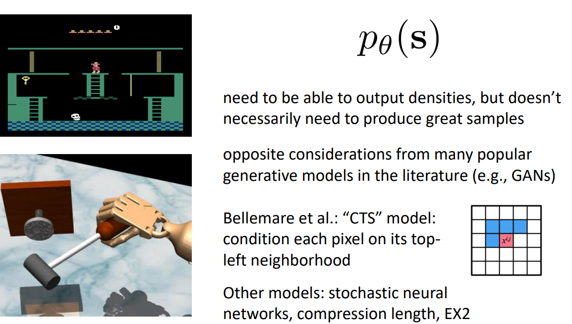
- Need to be able to output densities, but doesn’t necessarily need to produce great samples. Opposite considerations from many popular generative models in the literature (e.g., GANs)
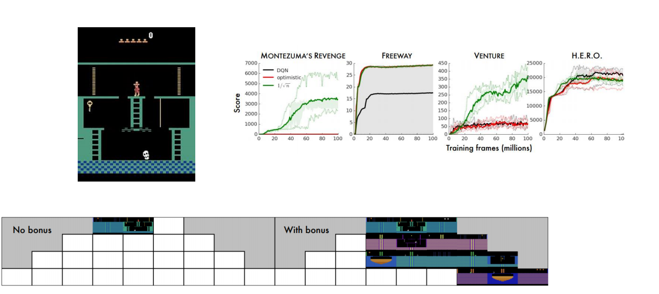
- Bellemare et al.: “CTS” model: condition each pixel on its topleft neighborhood
Different Bonus Versions:
Results:
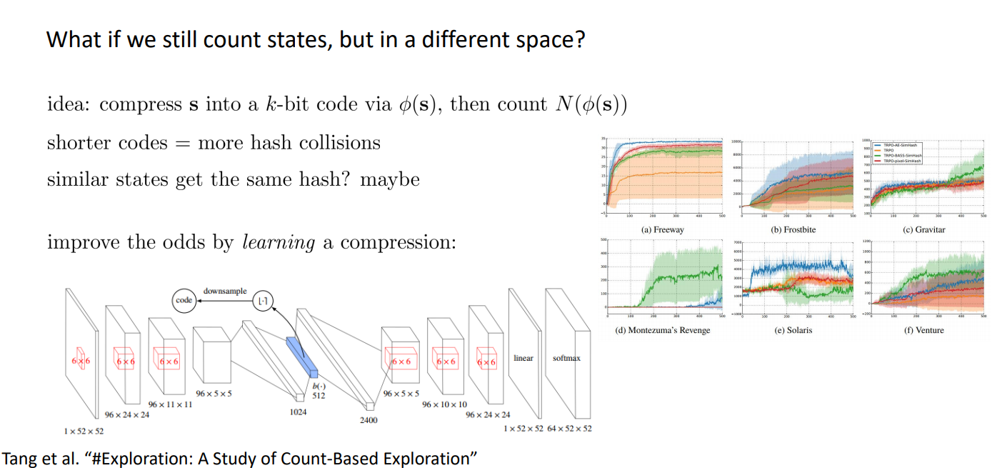
Counting with Hashes:
Idea: compress states into k-bit code via \(\phi(s)\), then count \(N(\phi(s))\)
Shorter codes = more hash collisions,
probably similar states get the same hash...
Improve the odds by learning a compression:

Implicit Density Modeling:
\(p_{\theta}(s)\) need to be able to output densities, but doesn’t necessarily need to produce great samples
Intuition: the state is novel if it is easy to distinguish from all previous seen states by a classifier
For each observation state \(s\), fit a classifier to classify that state against past states \(D\), use classifier error to obtain density:
p_{\theta}(s) = \frac{1 - D_s(s)}{D_s(s)}
probability that classifier assigns that \(s\) is not in past states \(D\)
Implicit Densities:
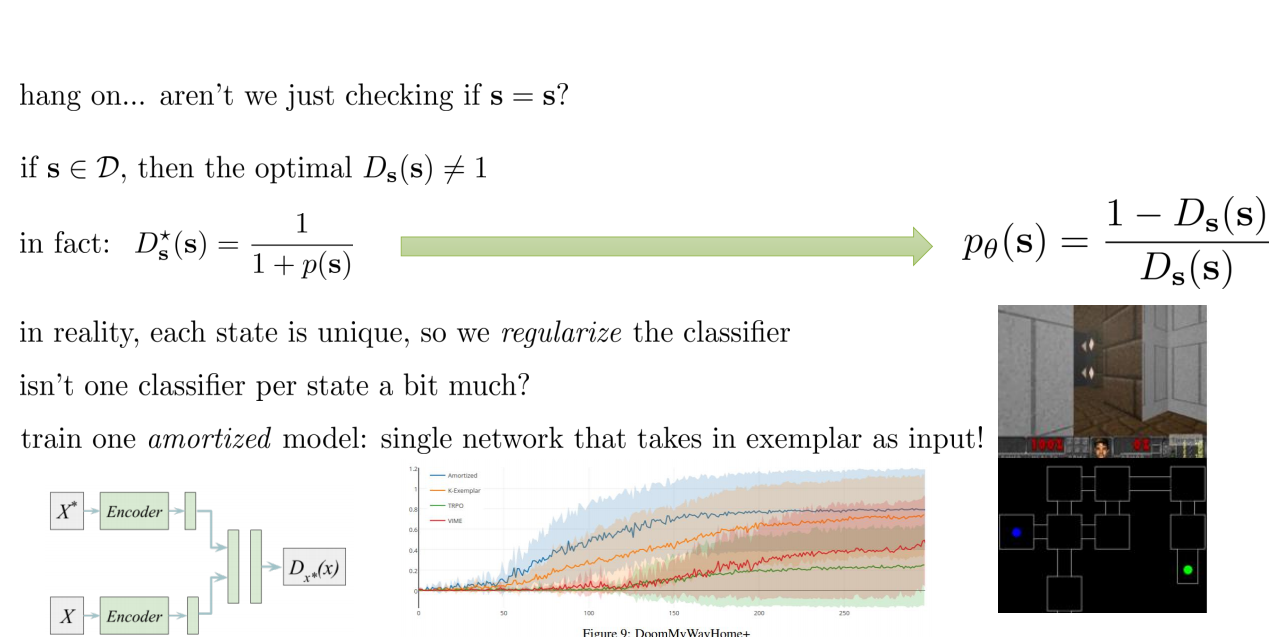
- if \(s \in D \), then the optimal \(D_s(s) \ne 1\)
- in fact \(D^{*}_s(s) = 1/(1 + p_{\theta}(s))\)
That is where we get:
Fitting a new classifier for each new state is abit to much,
therefore we train a single network that takes s as input:
p_{\theta}(s) = \frac{1 - D_s(s)}{D_s(s)}
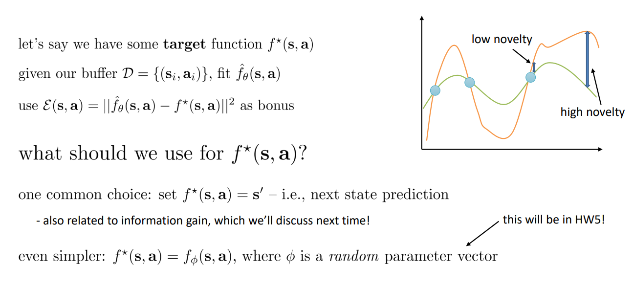
Heuristic estimation of counts via errors
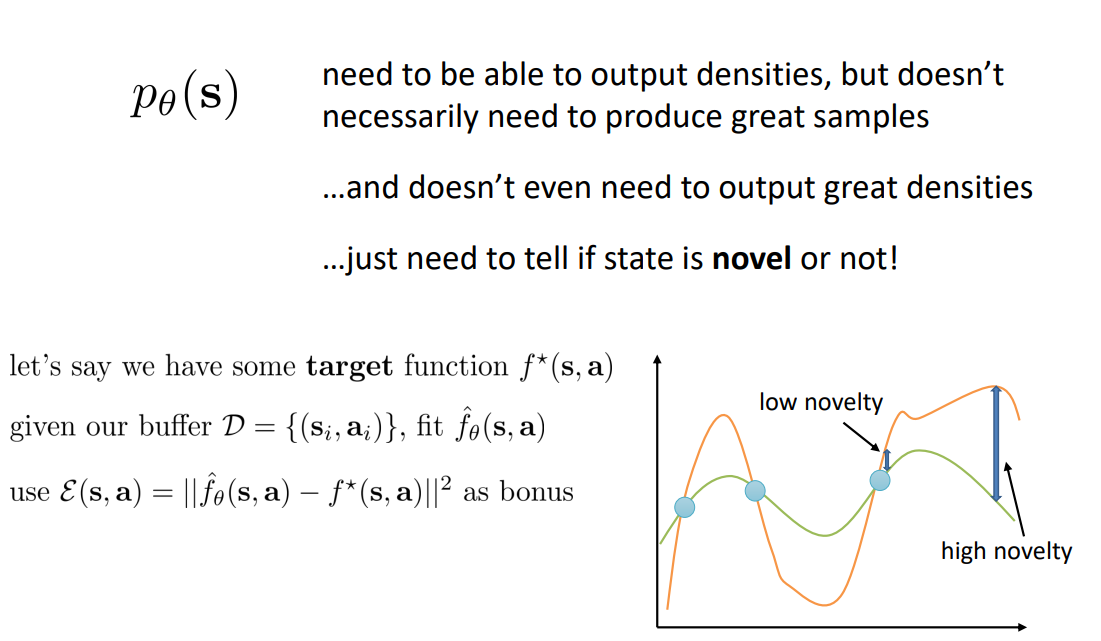
- \(p_{\theta}(s)\) need to be able to output densities, but doesn’t necessarily need to produce great samples
- And doesn’t even need to output great densities
- Just need to tell if state is novel or not!
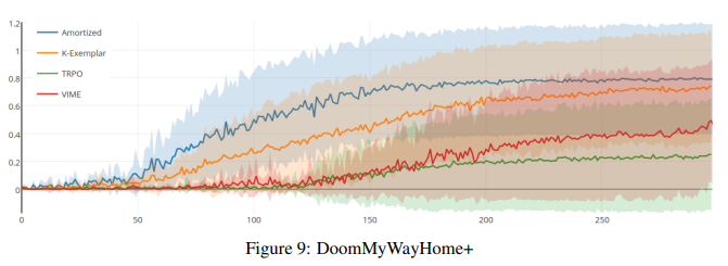
Heuristic estimation of counts via errors
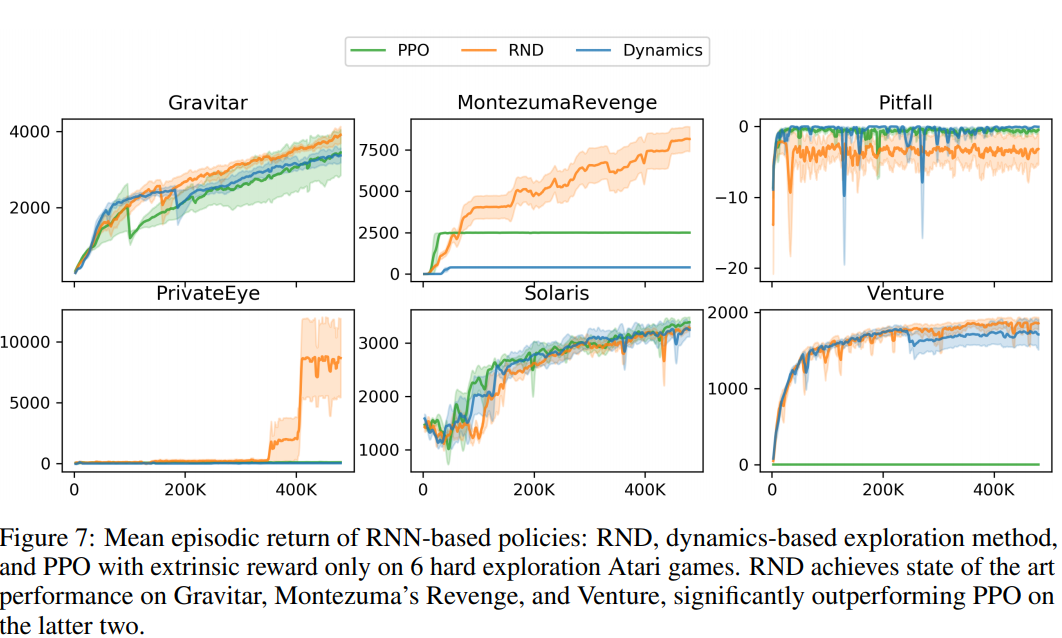
Random Network Distillation: Results
Thompson Sampling in Deep RL
Bootstrapped DQN
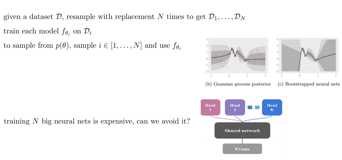
Bootstrapped DQN
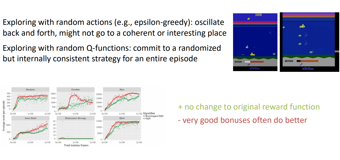
- Exploring with random actions (e.g., epsilon-greedy): oscillate back and forth, might not go to a coherent or interesting place
- Exploring with random Q-functions: commit to a randomized but internally consistent strategy for an entire episode

Information Gain in Deep RL....


Thank you for your attention!
12 - Exploration
By supergriver


