Dojo:
A differentiable simulator for robotics
Simon Le Cleac'h and Taylor Howell







Taylor Howell
Simon Le Cleac'h
Jan Brüdigam
Zico Kolter
Mac Schwager
Zachary Manchester
team

Dojo is a physics engine
that prioritizes
physical accuracy
and
differentiability


doesn't
MuJoCo/Drake/Bullet/Brax
already do that?


popular simulators
https://leggedrobotics.github.io/SimBenchmark/

github.com/dojo-sim
- Julia package: Dojo.jl
- Python wrapper: dojopy
- gym-like environments
- interface w/ PyTorch & JAX


- maximal-coordinates representation
- variational integrator
- higher-fidelity contact model
- custom interior-point solver
- smooth gradients
Dojo

maximal-coordinates representation


minimal-coordinates
representation

minimal-coordinates
representation

minimal-coordinates
representation

minimal-coordinates
representation

minimal-coordinates
representation

minimal-coordinates
representation

maximal-coordinates
representation

maximal-coordinates
representation

maximal-coordinates
representation

maximal-coordinates
representation

maximal-coordinates
representation

maximal-coordinates
representation

maximal-coordinates representation
Linear-Time Variational Integrators in Maximal Coordinates. J. Brudigam and Z. Manchester.
Linear-Time Contact and Friction Dynamics in Maximal Coordinates using Variational Integrators.
J. Brudigam and Z. Manchester.

variational integrator

variational integrator
Discrete mechanics and variational integrators. J. E. Marsden and M. West.
variational integrator
Discrete mechanics and variational integrators. J. E. Marsden and M. West.
Euler-Lagrange
variational integrator
Discrete mechanics and variational integrators. J. E. Marsden and M. West.
discretize
Euler-Lagrange
variational integrator
Discrete mechanics and variational integrators. J. E. Marsden and M. West.
discretize
discretize
Euler-Lagrange
variational integrator
Discrete mechanics and variational integrators. J. E. Marsden and M. West.
discretize
discretize
Euler-Lagrange
Euler-Lagrange
energy and momentum conservation

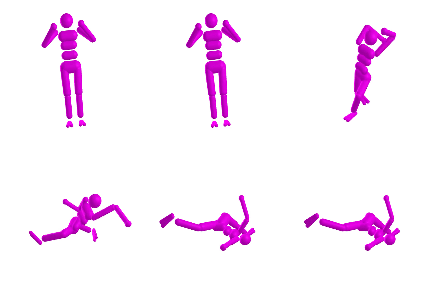
tennis-racket effect
astronaut
Simulation Tools for Model-Based Robotics: Comparison of Bullet, Havok, MuJoCo, ODE and PhysX.
T. Erez, Y. Tassa, and E. Todorov.
energy and momentum conservation

variational integrator
Euler:

contact model
floor penetration

drift
contact model
friction
On unilateral constraints, friction and plasticity. J. J. Moreau.

contact model
friction
On unilateral constraints, friction and plasticity. J. J. Moreau.

friction cones

approximation
exact
friction cones
Subtitle

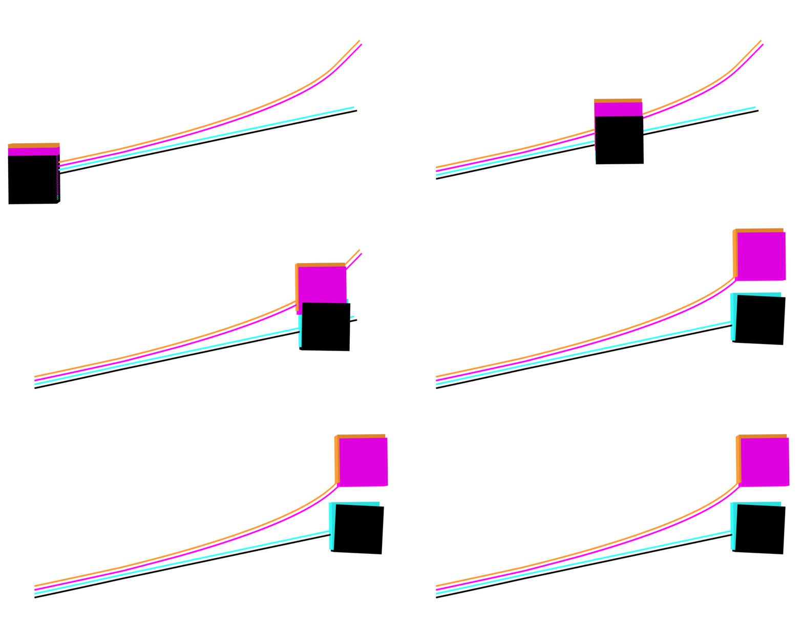

MuJoCo linear
Dojo linear
MuJoCo nonlinear
Dojo nonlinear
contact model
impact
An Implicit Time-Stepping Scheme for Rigid Body Dynamics with Inelastic Collisions and Coloumb Friction. D. E. Stewart and J. C. Trinkle.
contact model
impact
An Implicit Time-Stepping Scheme for Rigid Body Dynamics with Inelastic Collisions and Coloumb Friction. D. E. Stewart and J. C. Trinkle.
contact model
impact
An Implicit Time-Stepping Scheme for Rigid Body Dynamics with Inelastic Collisions and Coloumb Friction. D. E. Stewart and J. C. Trinkle.
contact model
impact
An Implicit Time-Stepping Scheme for Rigid Body Dynamics with Inelastic Collisions and Coloumb Friction. D. E. Stewart and J. C. Trinkle.
impact
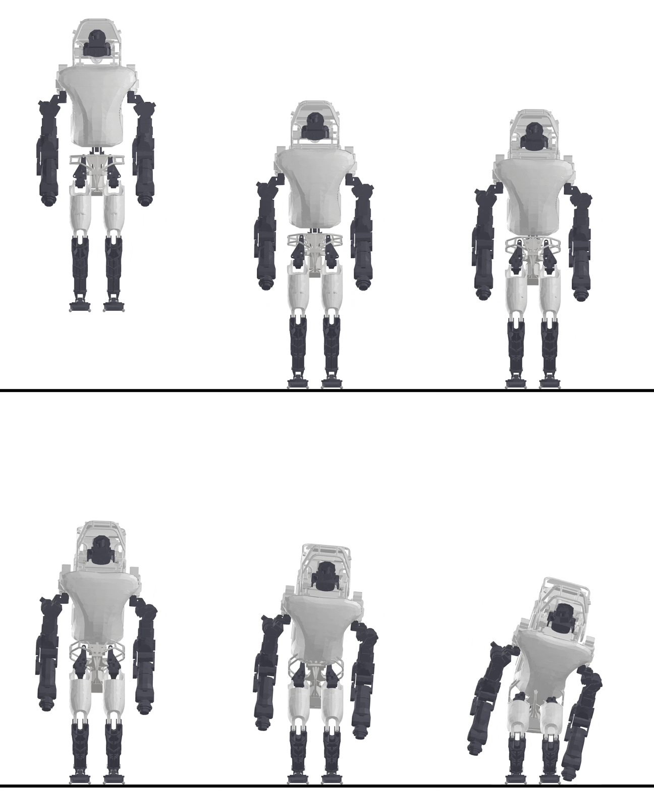
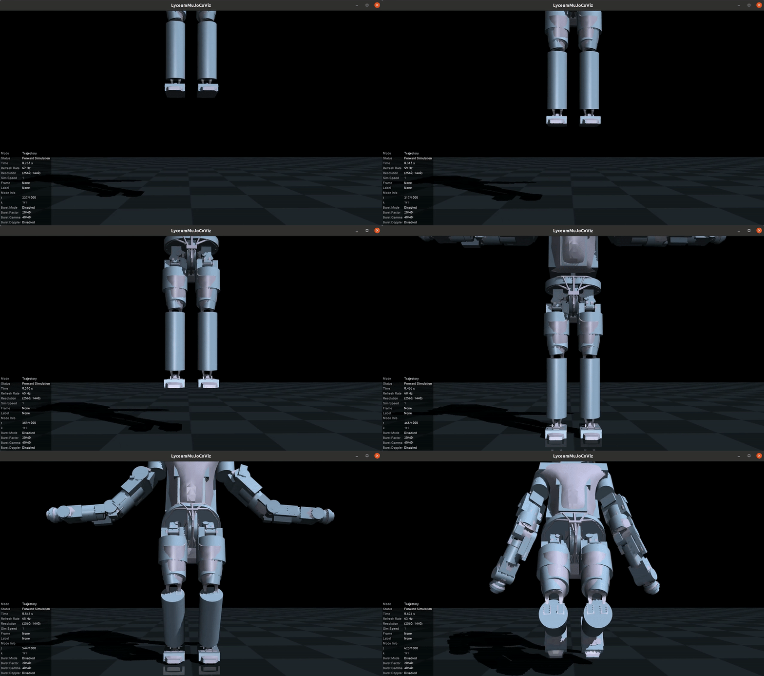
Dojo
MuJoCo

interior-point solver
interior-point solver
interior-point solver

interior-point solver


interior-point solver


interior-point solver

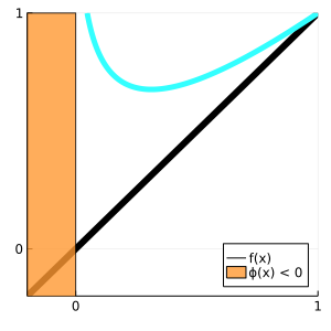
interior-point solver


interior-point solver
KKT conditions


interior-point solver
KKT conditions

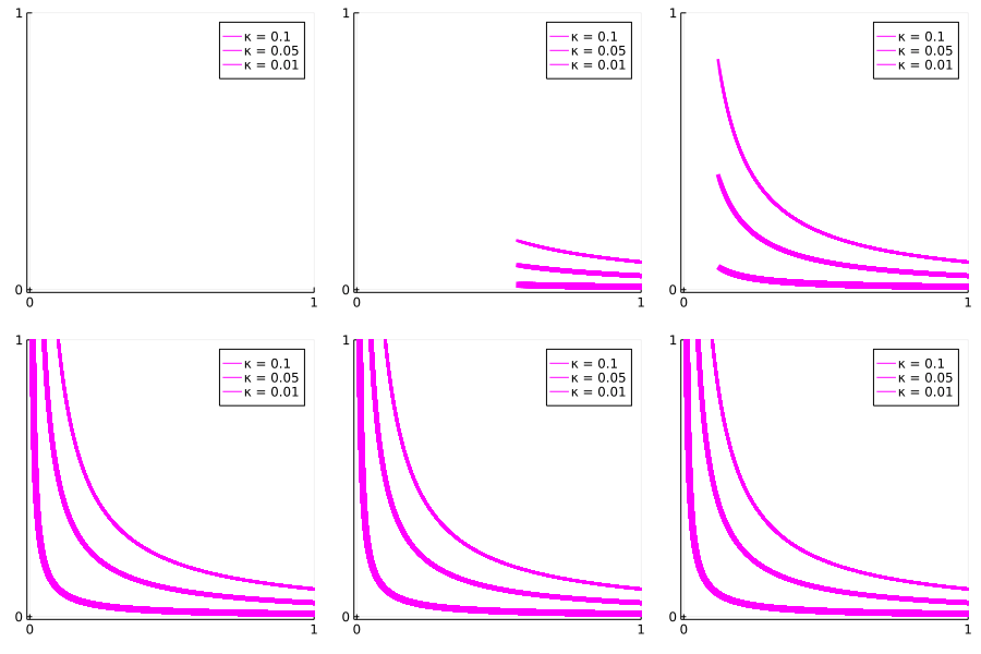
interior-point solver

interior-point solver

interior-point solver

using Plots
using Dojo

rectangle(w, h, x, y) = Shape(x .+ [0,w,w,0], y .+ [0,0,h,h])
light_blue = RGBA(0.4,0.4,1.0,0.8)

f(x) = x
ϕ(x) = x
L(x, ρ) = f(x) - ρ * log.(ϕ(x))
X = 0:0.0001:1
Y = -1:0.1:1
plt = plot(ylims=(-0.2,1.0), xlims=(-0.2,1.0), yticks=[0,1], xticks=[0,1], legend=:bottomright, size=(300,300))
plot!(plt, Y, f.(Y), linewidth=6.0, color=:black, label="f(x)")
plot!(rectangle(-0.2,2,0,-1), opacity=.6, color=:red, label="ϕ(x) < 0")
anim = @animate for i = 1:10
    plot!(plt, X, [1; L.(X[2:end], 10*0.5^i)], linewidth=5.0, color=light_blue, label=false)# label="ρ = 3e-1")
end
gif(anim, fps=10, "/home/simon/Downloads/anim.gif")

PHI = Vector(1:-0.005:0)
plt = plot(ylims=(-0.01,1.0), xlims=(-0.01,1.0), yticks=[0,1], xticks=[0,1], legend=:topright, size=(300,300), )
anim = @animate for i = 1:440
    # for (j,κ) ∈ enumerate([1e-1, 5e-2, 1e-2])
    for (j,κ) ∈ enumerate([5e-2,])
        PHI_i = PHI[1:min(i,length(PHI))]
        (i == 1) && plot!(plt, PHI_i, κ ./ PHI_i, color=light_blue, linewidth=1+1.5j, label="κ = $κ")
        plot!(plt, PHI_i, κ ./ PHI_i, color=light_blue, linewidth=1+1.5j, label=nothing)
    end
end

gif(anim, fps=40, "/home/simon/Downloads/force_solo.gif")

plot!(plt, PHI, 1e-2 ./ PHI, color=light_blue, linewidth=5.0, label="κ = 1e-2")
plot!(plt, PHI, 1e-3 ./ PHI, color=light_blue, linewidth=5.0, label="κ = 1e-3")
gradients
gradients
gradients

gradients

gradients

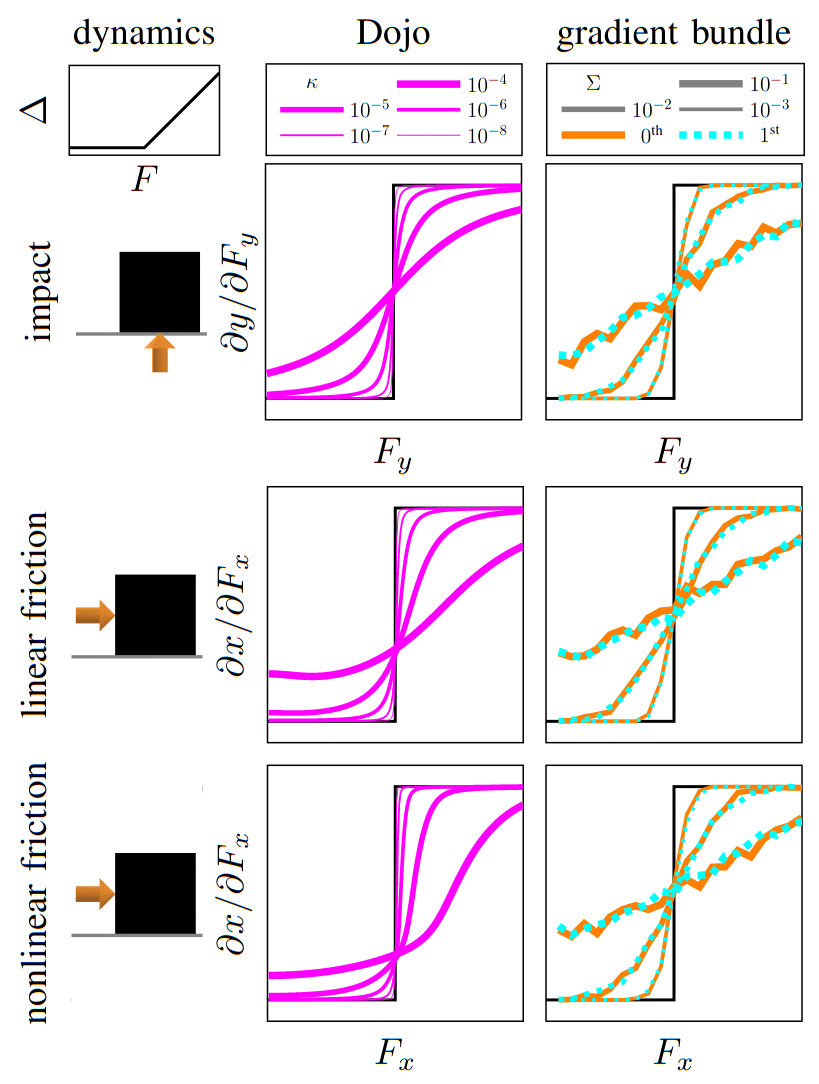
gradients
implicit-function theorem
Lezioni di analisi infinitesimale. U. Dini.
gradients

implicit-function theorem
Lezioni di analisi infinitesimale. U. Dini.
gradients

implicit-function theorem
Lezioni di analisi infinitesimale. U. Dini.
solution
gradients

implicit-function theorem
Lezioni di analisi infinitesimale. U. Dini.
solution
residual
gradients

implicit-function theorem
Lezioni di analisi infinitesimale. U. Dini.
solution
data
residual
trajectory optimization


Dojo: success
MuJoCo: success
Dojo: success
MuJoCo: failure
gradients

examples
trajectory optimization

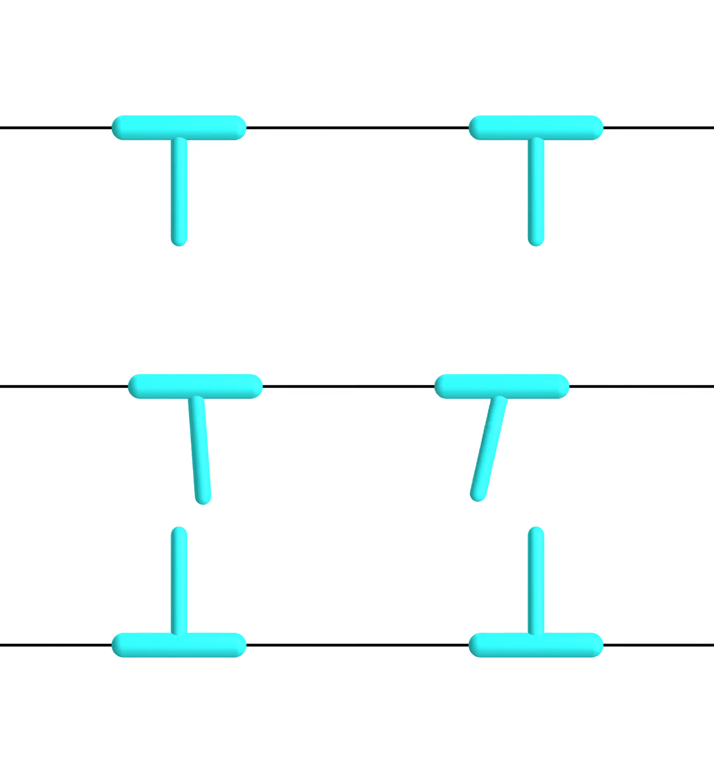
optimized with iterative LQR
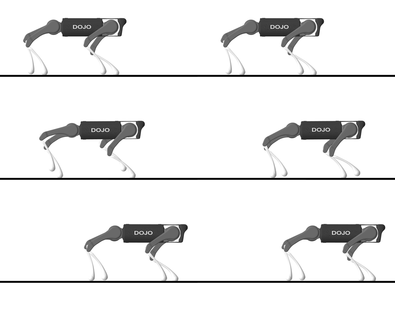
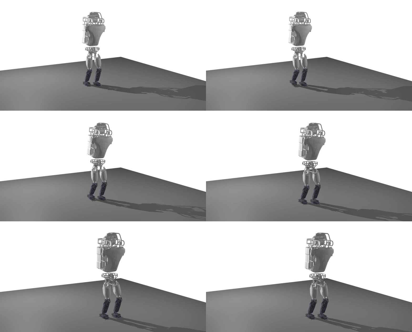
reinforcement learning
Subtitle

augmented random search to train static linear policies
reinforcement learning

augmented random search v. augmented gradient search
system identification
ContactNets: Learning Discontinuous Contact Dynamics with Smooth, Implicit Representations.
S. Pfrommer, M. Halm, and M. Posa.

system identification
ContactNets: Learning Discontinuous Contact Dynamics with Smooth, Implicit Representations.
S. Pfrommer, M. Halm, and M. Posa.
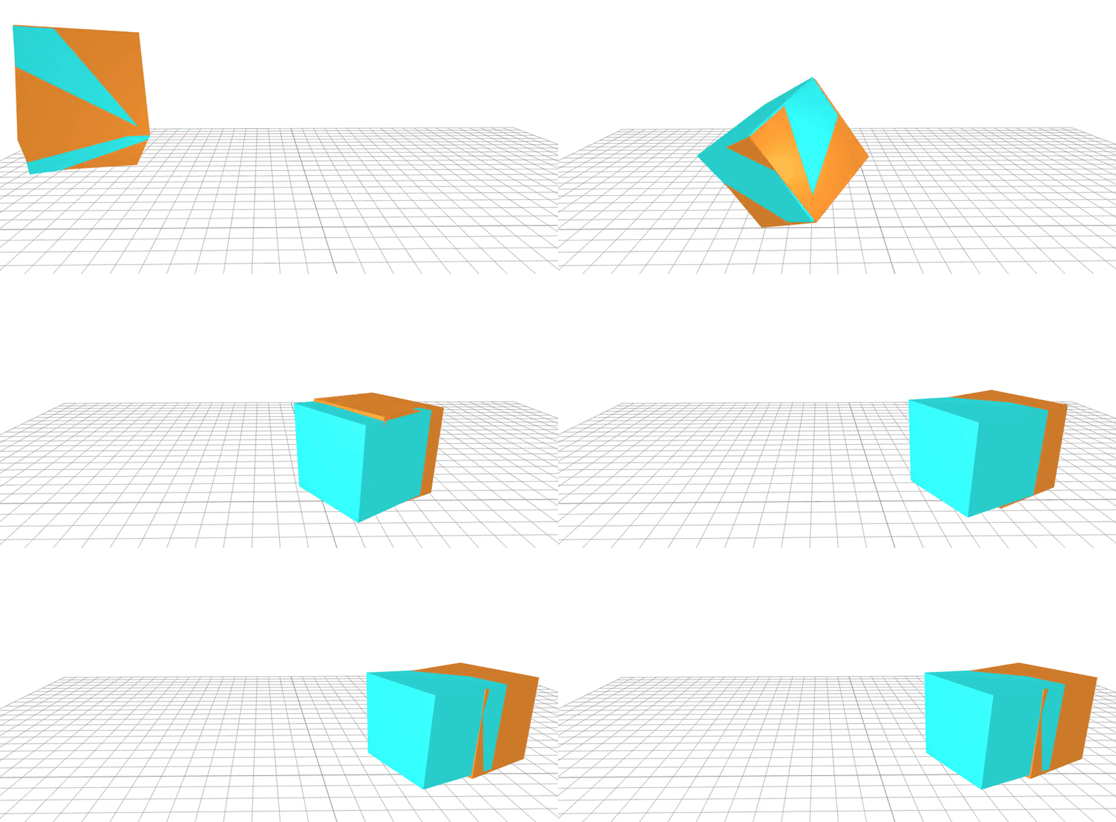
learned
ground-truth
system identification
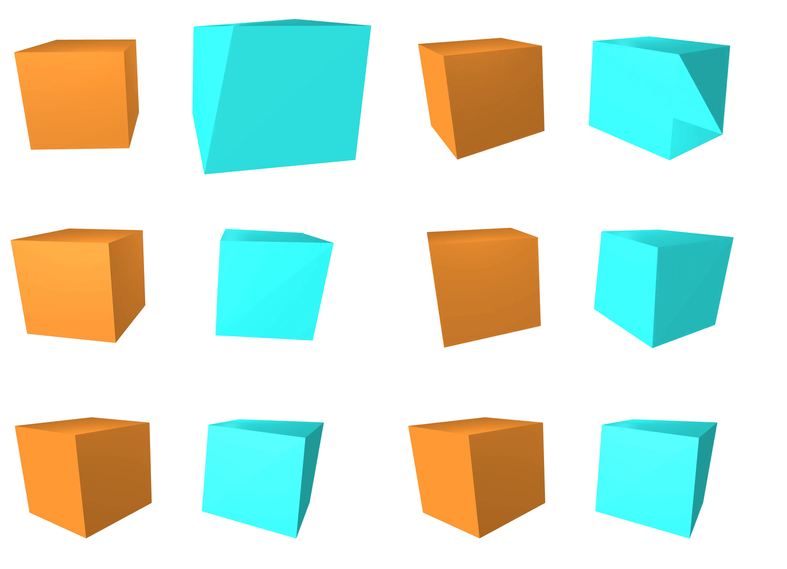
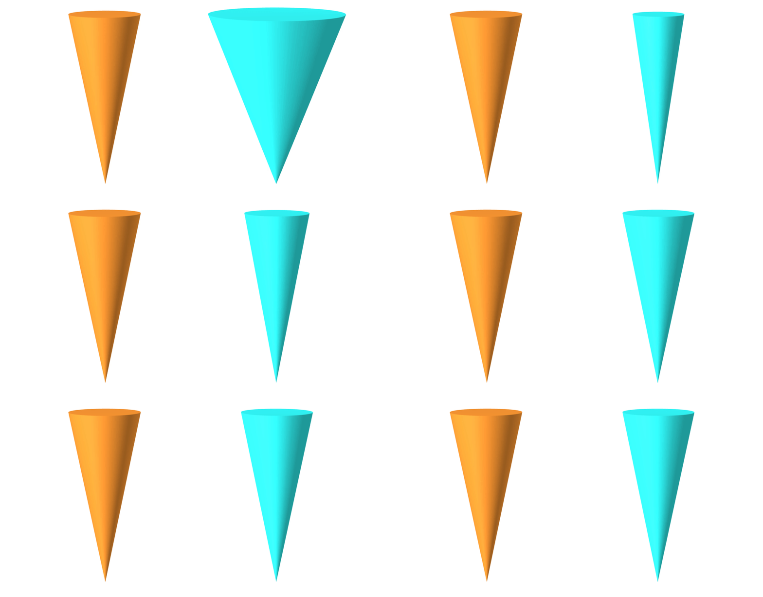
learning via quasi-Newton method
geometry
friction coefficient
ground-truth
learned
system identification

system identification


Dojo gradient
live demo

model-predictive control

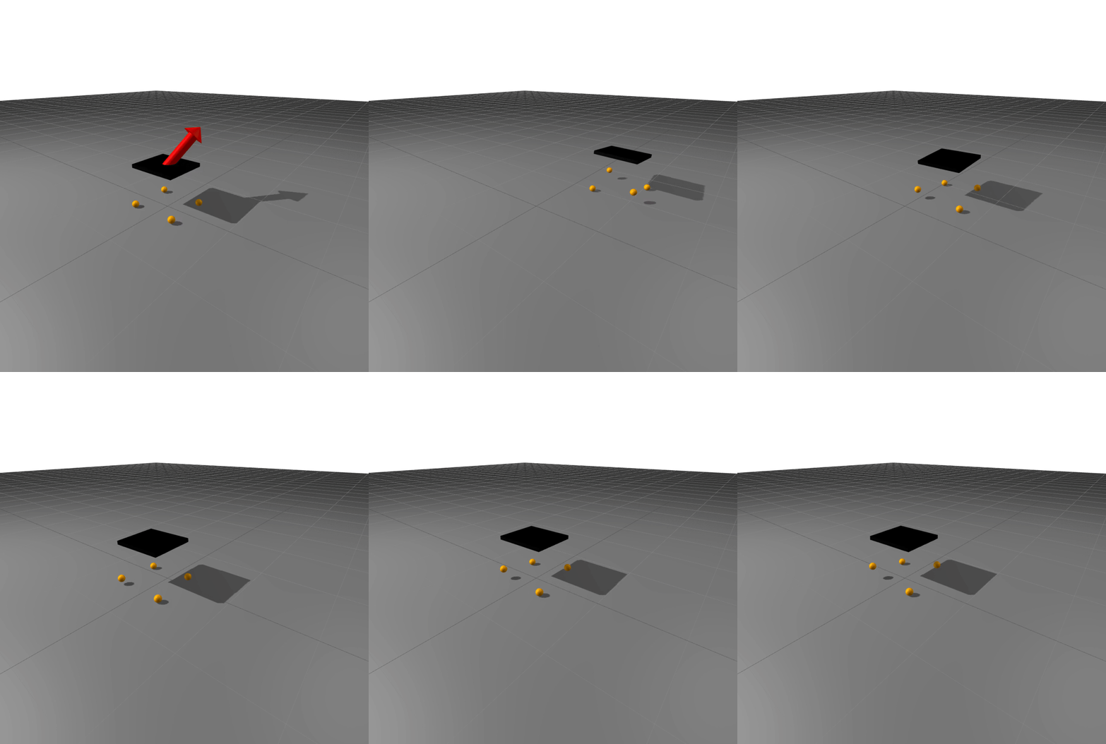
model-predictive control


model-predictive control


model-predictive control


NeRF


fast policy learning


github.com/dojo-sim
Dojo: A differentiable simulator for robotics
By taylorhowell
Dojo: A differentiable simulator for robotics
- 522


