H.J. Terry Suh, MIT
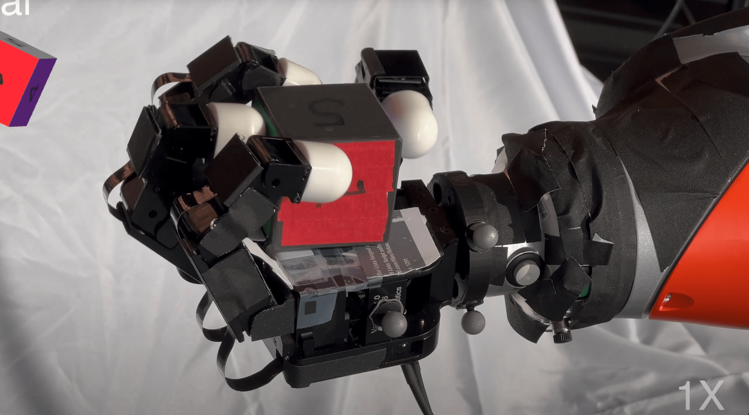
Leveraging Structure for Efficient and Dexterous Contact-Rich Manipulation
[TRO 2023, TRO 2025]
Part 3. Global Planning for Contact-Rich Manipulation
Part 2. Local Planning / Control via Dynamic Smoothing
Part 1. Understanding RL with Randomized Smoothing
Introduction
[TRO 2023, TRO 2025]
Introduction
Why contact-rich manipulation?
What has been done, and what's lacking?
What is manipulation?
How hard could this be? Just pick and place!
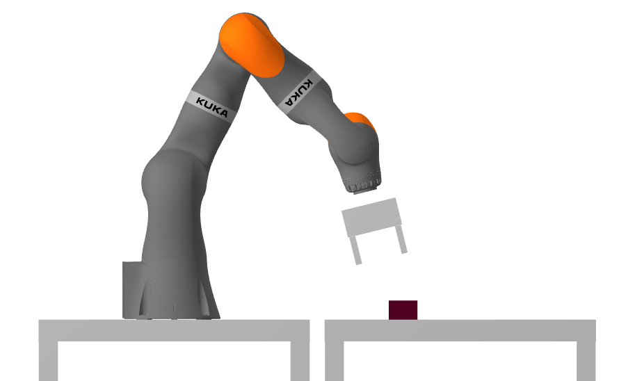
Rigid-body manipulation: Move object from pose A to pose B

A
B
Manipulation is NOT pick & place


[ZH 2022]
[SKPMAT 2022]
[PSYT 2022]
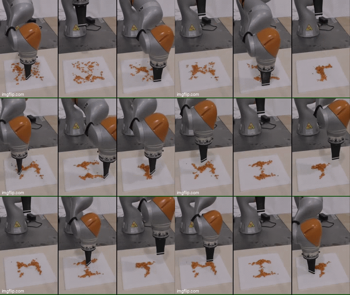
[ST 2020]
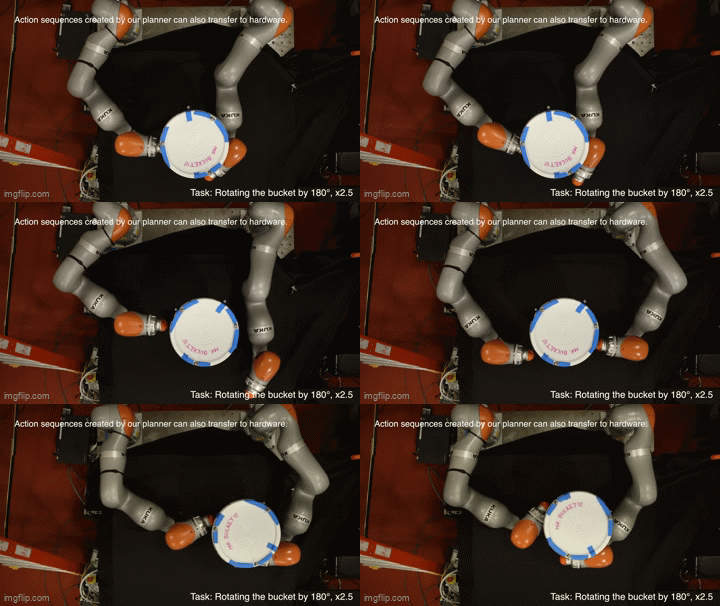

Manipulation: An Important Problem

Matt Mason, "Towards Robotic Manipulation", 2018
Manipulation: An Important Problem

Matt Mason, "Towards Robotic Manipulation", 2018
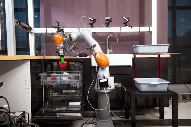
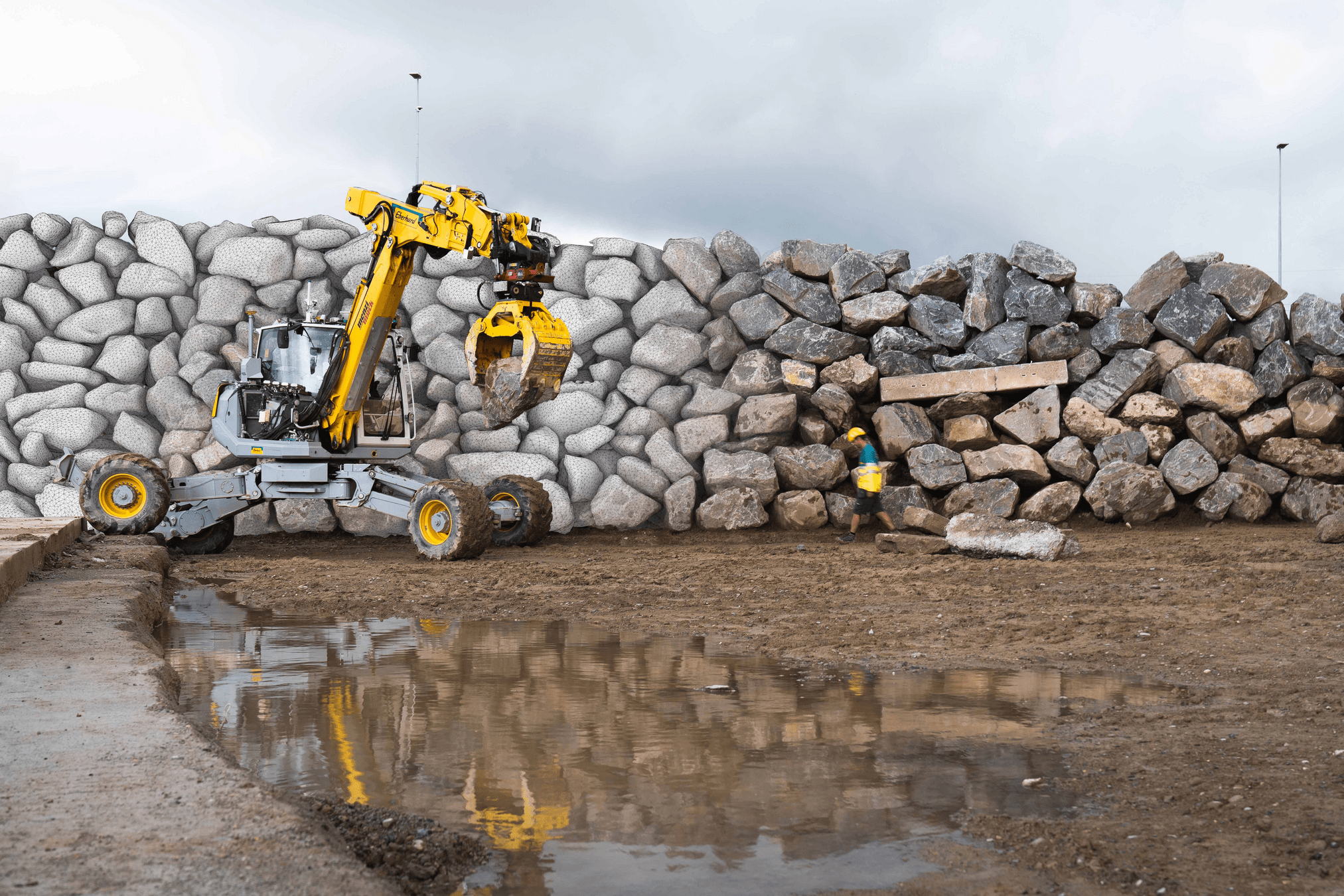
Manipulation is a core capability for robots to broaden the spectrum of things we can automate in this world.


DexAI
TRI Dishwasher Demo
Flexxbotics
ETH Zurich, Robotic Systems Lab
What is Contact-Rich Manipulation?
Why should there be an inherent value in studying
manipulation that is rich in contact?
What is Contact-Rich Manipulation?
Why should there be an inherent value in studying
manipulation that is rich in contact?

Matt Mason, "Towards Robotic Manipulation", 2018
Manipulation
What is Contact-Rich Manipulation?

Matt Mason, "Towards Robotic Manipulation", 2018
Manipulation
What is Contact-Rich Manipulation?

Matt Mason, "Towards Robotic Manipulation", 2018
Manipulation
What is Contact-Rich Manipulation?

Matt Mason, "Towards Robotic Manipulation", 2018
Manipulation
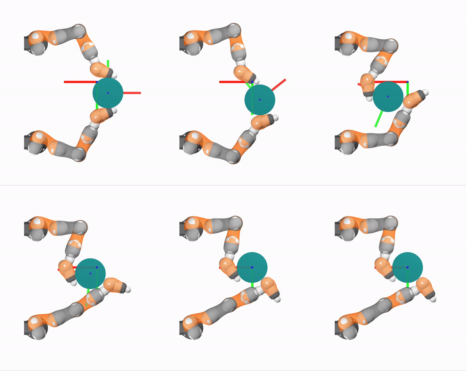
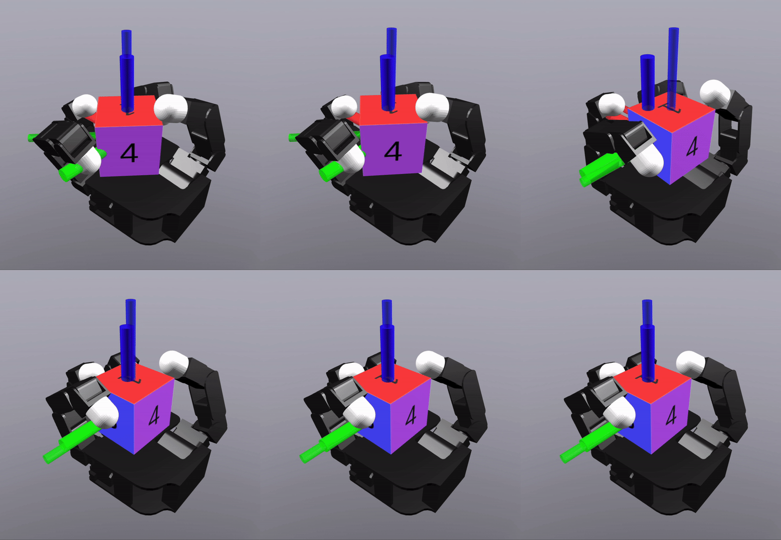
- Where do I make contact?
- Where should I avoid contact?
- With what timing?
- What do I do after making contact?
What is Contact-Rich Manipulation?

Matt Mason, "Towards Robotic Manipulation", 2018
Manipulation


- Where do I make contact?
- Where should I avoid contact?
- With what timing?
- What do I do after making contact?
As possibilities become many, strategic decisions become harder.
What is Contact-Rich Manipulation?
Manipulation
Manipulation that strategically makes decisions about contact after considering multiple possible ways of selecting contact, especially when such possibilities are many.
Contact-Rich Manipulation
H.J. Terry Suh, PhD Thesis

Matt Mason, "Towards Robotic Manipulation", 2018
What is Contact-Rich Manipulation?
Manipulation
Manipulation that strategically makes decisions about contact after considering multiple possible ways of selecting contact, especially when such possibilities are many.
Contact-Rich Manipulation
H.J. Terry Suh, PhD Thesis

Matt Mason, "Towards Robotic Manipulation", 2018
- Doesn't necessarily have to behaviorally result in many contacts.
What is Contact-Rich Manipulation?
Manipulation
Manipulation that strategically makes decisions about contact after considering multiple possible ways of selecting contact, especially when such possibilities are many.
Contact-Rich Manipulation
H.J. Terry Suh, PhD Thesis

Matt Mason, "Towards Robotic Manipulation", 2018
- Doesn't necessarily have to behaviorally result in many contacts.
- Shouldn't artificially restrict possible contacts from occuring.
Case 1. Whole-Body Manipulation

Do not make contact
(Collision-free Motion Planning)
Make Contact
Human
Robot
Slide inspired by Tao Pang's Thesis Defense & TRI Punyo Team

Case 2. Dexterous Manipulation
Human
Robot
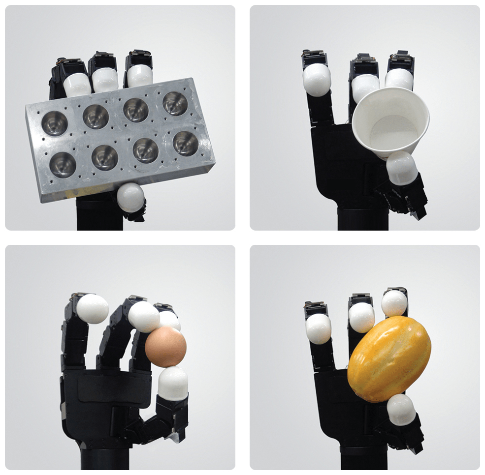
Wonik Allegro Hand
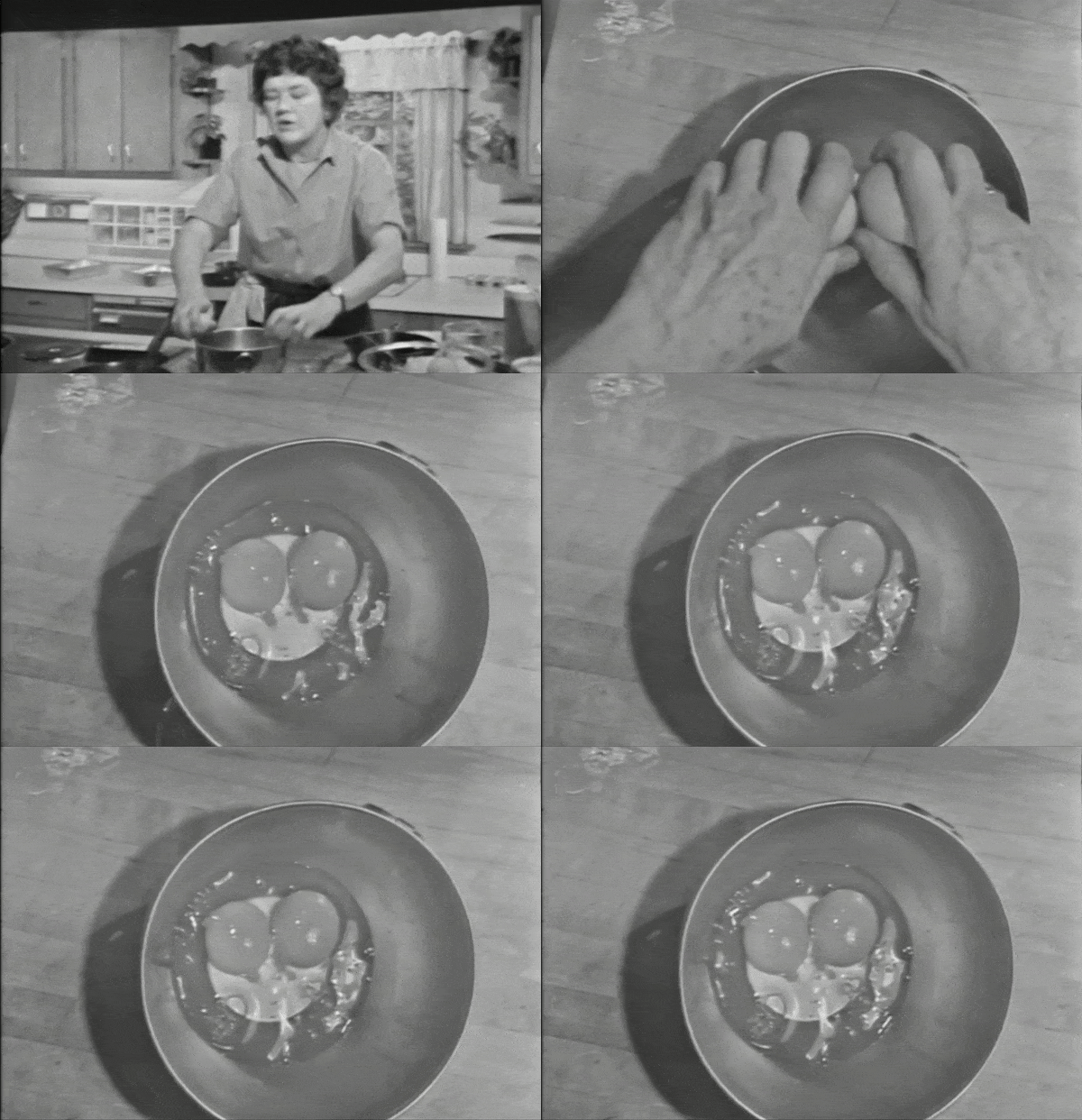
Why Contact-Rich Manipulation?
A capable embodied intelligence must be able to exploit its physical embodiment to the fullest.
Manipulation that strategically makes decisions about contact after considering multiple possible ways of selecting contact, especially when such possibilities are many.
Contact-Rich Manipulation
H.J. Terry Suh, PhD Thesis
[TRO 2023, TRO 2025]
Introduction
Why contact-rich manipulation?
What has been done, and what's lacking?


[TRO 2023, TRO 2025]
Introduction
What has been done, and what's lacking?
Why contact-rich manipulation?


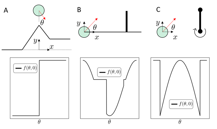
Fundamental Challenges
Cost
Cost
Cost

Fundamental Challenges
Flatness and Stiffness spells difficulty for local gradient-based optimizers.
Cost
Cost
Cost
Smooth Analysis

But GIVEN a contact event, the landscape is smooth.
Cost
Cost
Cost
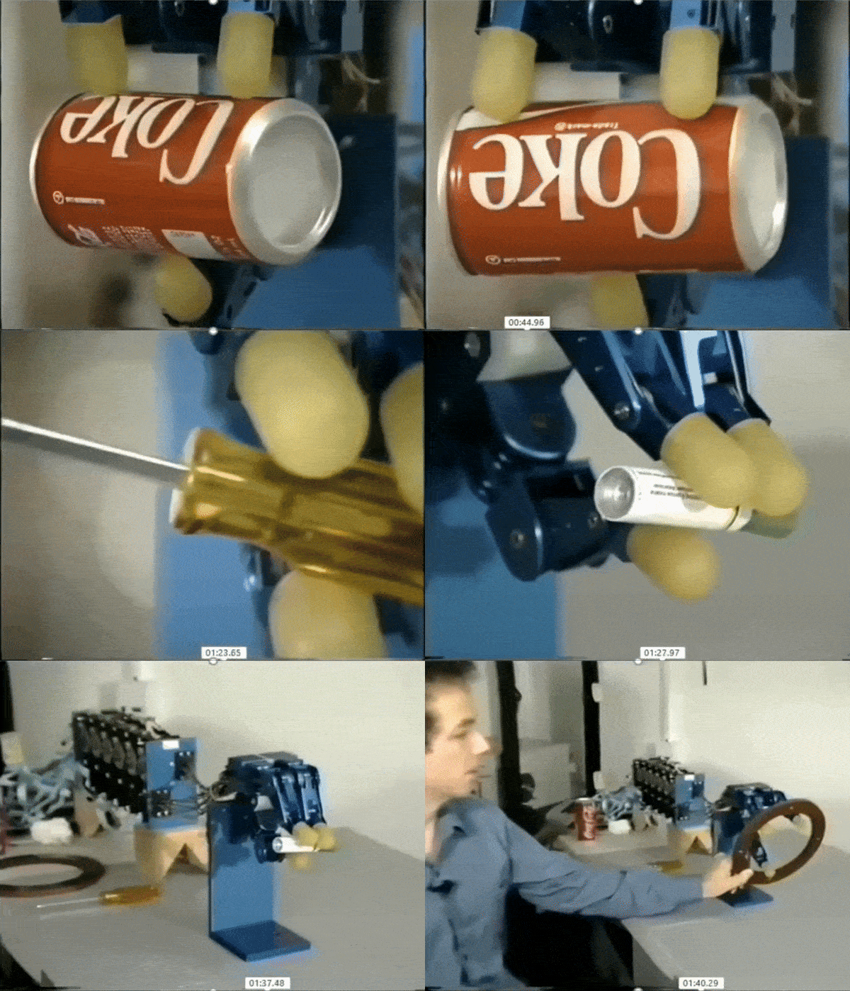
[Salisbury Hand, 1982]
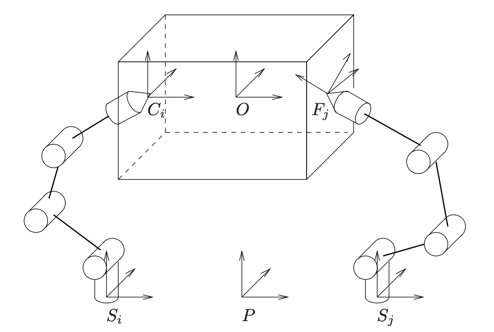
[Murray, Li, Sastry]
What can we do given a contact mode?
Smooth Planning & Control
Combinatorial Optimization

Cost
Cost
Cost
Can we try to globally search for the right "piece"?
Hybrid Dynamics & Combinatorial Optimization
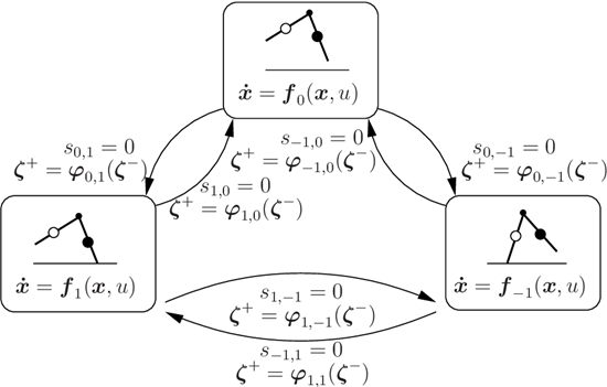
Contact dynamics as a "hybrid system" with continuous and discrete components.
[Sreenath et al., 2009]
Hybrid Dynamics & Combinatorial Optimization
[Hogan et al., 2009]
[Graesdal et al., 2024]
Beautiful results in locomotion & manipulation
Problems with Mode Enumeration
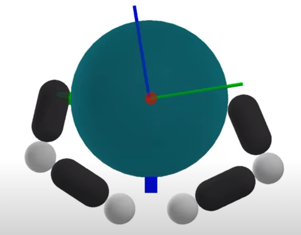
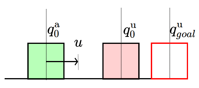
System
Number of Modes
No Contact
Sticking Contact
Sliding Contact
Number of potential active contacts
Problems with Mode Enumeration


System
Number of Modes
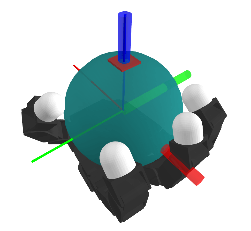
The number of modes scales terribly with system complexity
No Contact
Sticking Contact
Sliding Contact
Number of potential active contacts
Contact Relaxation & Smooth NLP
[Posa et al., 2015]
[Mordatch et al., 2012]
Reinforcement Learning
[OpenAI et al., 2019]
[Handa et al., 2024]
Reinforcement Learning
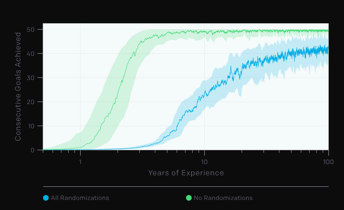
[OpenAI et al., 2019]
Summary of Previous Approaches
Classical Mechanics
Contact Scalability
Efficiency
Global Scope


Summary of Previous Approaches
Classical Mechanics
Hybrid Dynamics &
Combinatorial Optimization
Contact Scalability
Efficiency
Global Scope


Summary of Previous Approaches
Classical Mechanics
Hybrid Dynamics &
Combinatorial Optimization
Contact Relaxation &
Smooth Nonlinear Programming
Contact Scalability
Efficiency
Global Scope


Summary of Previous Approaches
Classical Mechanics
Hybrid Dynamics &
Combinatorial Optimization
Contact Relaxation &
Smooth Nonlinear Programming
Reinforcement Learning
Contact Scalability
Efficiency
Global Scope


Summary of Previous Approaches
Classical Mechanics
Hybrid Dynamics &
Combinatorial Optimization
Contact Relaxation &
Smooth Nonlinear Programming
Reinforcement Learning
Contact Scalability
Efficiency
Global Scope


How can we achieve all three criteria?
Introduction
What has been done, and what's lacking?
Why contact-rich manipulation?


Part 3. Global Planning for Contact-Rich Manipulation
Part 2. Local Planning / Control via Dynamic Smoothing
Part 1. Understanding RL with Randomized Smoothing

Introduction

Preview of Results
Our Method


Contact Scalability
Efficiency
Global Planning

60 hours, 8 NVidia A100 GPUs
5 minutes, 1 Macbook CPU

[TRO 2023, TRO 2025]
Part 3. Global Planning for Contact-Rich Manipulation
Part 2. Local Planning / Control via Dynamic Smoothing
Part 1. Understanding RL with Randomized Smoothing

Introduction

[TRO 2023, TRO 2025]
Part 1. Understanding RL with Randomized Smoothing
Why does RL
perform well?
Why is it considered inefficient?
Can we do better with more structure?
[RA-L 2021, ICML 2022]
[TRO 2023, TRO 2025]
Part 1. Understanding RL with Randomized Smoothing
Why does RL
perform well?
Why is it considered inefficient?
Can we do better with more structure?
[RA-L 2021, ICML 2022]
How does RL search through these difficult problems?
Original Problem

[ICML 2022]
Cost
Cost
Cost
How does RL search through these difficult problems?
Randomized Smoothing
[ICML 2022]

How does RL search through these difficult problems?
Randomized Smoothing
[ICML 2022]

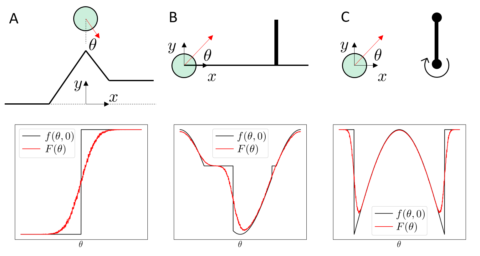
Noise regularizes difficult landscapes,
allevates flatness and stiffness,
abstracts contact modes.
[TRO 2023, TRO 2025]
Part 1. Understanding RL with Randomized Smoothing
Why does RL
perform well?
Why is it considered inefficient?
Can we do better with more structure?
[RA-L 2021, ICML 2022]

How does RL search through these difficult problems?
Randomized Smoothing
[ICML 2022]

But how do we take gradients of a stochastic function?
Estimation of Gradients with Monte Carlo
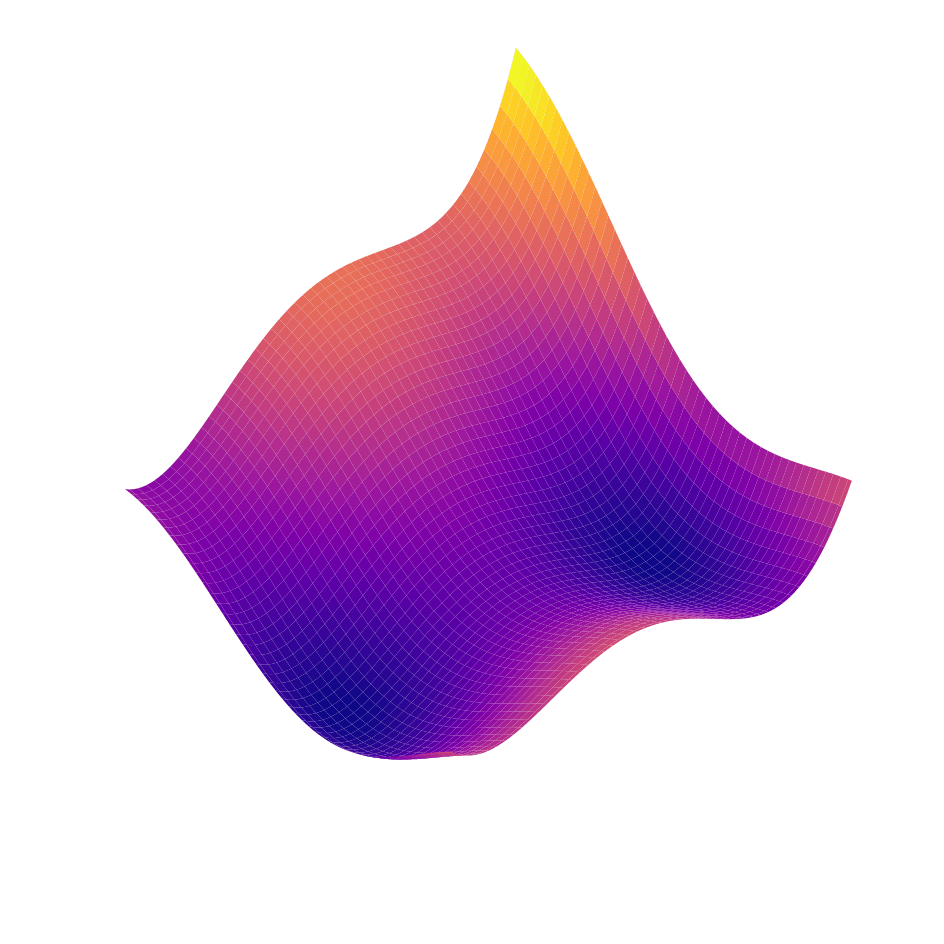
Zeroth-Order Gradient Estimator
- Stein Gradient Estimator
- REINFORCE
- Score Function / Likelihood Ratio Estimator
Estimation of Gradients with Monte Carlo
Zeroth-Order Gradient Estimator
- Stein Gradient Estimator
- REINFORCE
- Score Function / Likelihood Ratio Estimator
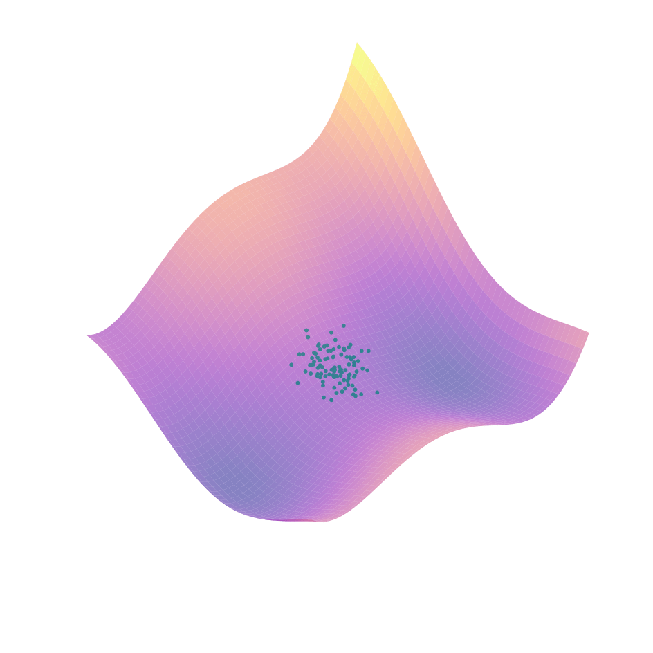
Estimation of Gradients with Monte Carlo

Zeroth-Order Gradient Estimator
- Stein Gradient Estimator
- REINFORCE
- Score Function / Likelihood Ratio Estimator
Estimation of Gradients with Monte Carlo

Zeroth-Order Gradient Estimator
- Stein Gradient Estimator
- REINFORCE
- Score Function / Likelihood Ratio Estimator
But what if we had access to gradients?
Leveraging Differentiable Physics
First-Order Randomized Smoothing
- Gradient Sampling Algorithm
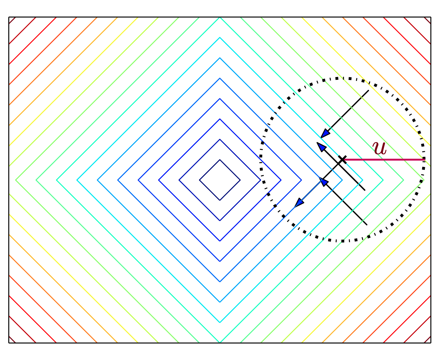
From John Duchi's Slides on Randomized Smoothing, 2014
Leveraging Differentiable Physics
First-Order Randomized Smoothing
- Gradient Sampling Algorithm

From John Duchi's Slides on Randomized Smoothing, 2014
So which one should we use?
Comparison of Efficiency
Bias
Variance
First-Order Estimator
Zeroth-Order Estimator


Comparison of Efficiency
Analytic Expression
First-Order Gradient Estimator
Zeroth-Order Gradient Estimator
- Requires differentiability over dynamics
- Generally lower variance.
- Least requirements (blackbox)
- High variance.
Possible for only few cases
Structure
Efficiency


[TRO 2023, TRO 2025]
Part 1. Understanding RL with Randomized Smoothing
Why does RL
perform well?
Why is it considered inefficient?
Can we do better with more structure?
[RA-L 2021, ICML 2022]

Bias
Variance
First-Order Estimator
Zeroth-Order Estimator
Comparison of Efficiency
Analytic Expression
First-Order Gradient Estimator
Zeroth-Order Gradient Estimator
- Requires differentiability over dynamics
- Generally lower variance.
- Least requirements (blackbox)
- High variance.
Possible for only few cases
Structure
Efficiency


Can we transfer this promise to RL?
Leveraging Differentiable Physics

Do Differentiable Simulators Give Better Gradients?
Leveraging Differentiable Physics

Do Differentiable Simulators Give Better Gradients?
Bias of First-Order Estimation
Bias of First-Order Estimation
Bias of First-Order Estimation

Bias of First-Order Estimation
Variance of First-Order Estimation
First-order Estimators CAN have more variance than zeroth-order ones.

Variance of First-Order Estimation

- No force when not in contact
- Spring-damper behavior when in contact
Variance of First-Order Estimation

- No force when not in contact
- Spring-damper behavior when in contact
Variance of First-Order Estimation

- No force when not in contact
- Spring-damper behavior when in contact
Prevalent for models that approximate contact through spring-dampers!
Gradients

Gradients
Bias
Variance
Common lesson from stochastic optimization:
1. Both are unbiased under sufficient regularity conditions
2. First-order generally has less variance than zeroth order.
Bias
Variance
Bias
Variance
1st Pathology: First-Order Estimators CAN be biased.
2nd Pathology: First-Order Estimators can have MORE
variance than zeroth-order.
Stiffness still hurts us in improving performance and efficiency
[TRO 2023, TRO 2025]
Part 1. Understanding RL with Randomized Smoothing
Why does RL
perform well?
Why is it considered inefficient?
Can we do better with more structure?
[RA-L 2021, ICML 2022]

Bias
Variance
First-Order Estimator
Zeroth-Order Estimator
Bias
Variance
First-Order Estimator
Zeroth-Order Estimator
[TRO 2023, TRO 2025]
Part 3. Global Planning for Contact-Rich Manipulation
Part 2. Local Planning / Control via Dynamic Smoothing
Part 1. Understanding RL with Randomized Smoothing

Introduction

[TRO 2023, TRO 2025]
Part 2. Local Planning / Control via Dynamic Smoothing
Can we do better by understanding dynamics structure?
How do we build effective local optimizers for contact?
Utilizing More Structure

- No force when not in contact
- Spring-damper behavior when in contact
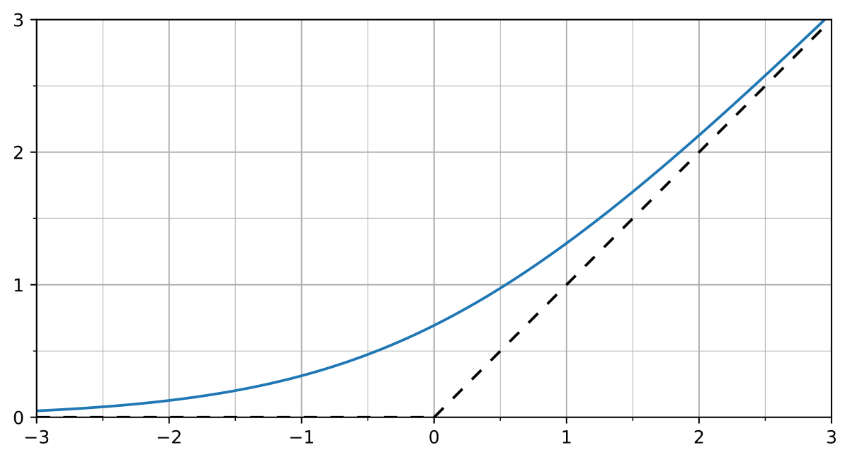
Tackling stiffness requires us to rethink about the models we use to simulate contact
Intuitive Physics of Contact
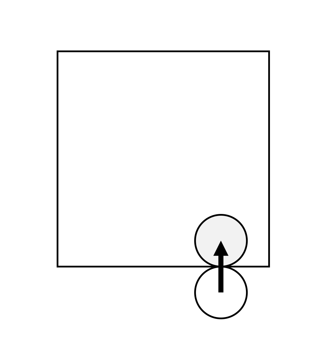
Where will the box move next?
Intuitive Physics of Contact


How did we know? Did we really have to integrate stiff springs?
Intuitive Physics of Contact
Intuitive Physics of Contact


How did we know? Did we really have to integrate stiff springs?
Constraint-Driven Simulations can simulate longer horizon behavior
Intuitive Physics of Contact
Intuitive Physics of Contact
Intuitive Physics of Contact


Did we think about velocities at all? Or purely reason about configuration?
Quasistatic Modeling & Optimization-Based Sim.
Optimization-Based Simulation
Quasistatic Modeling
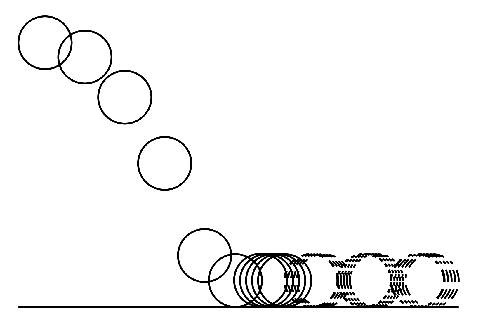
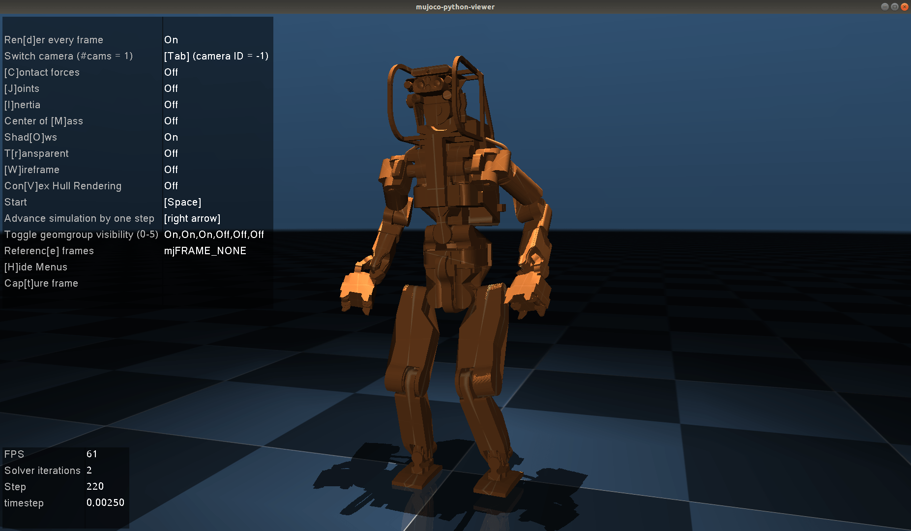
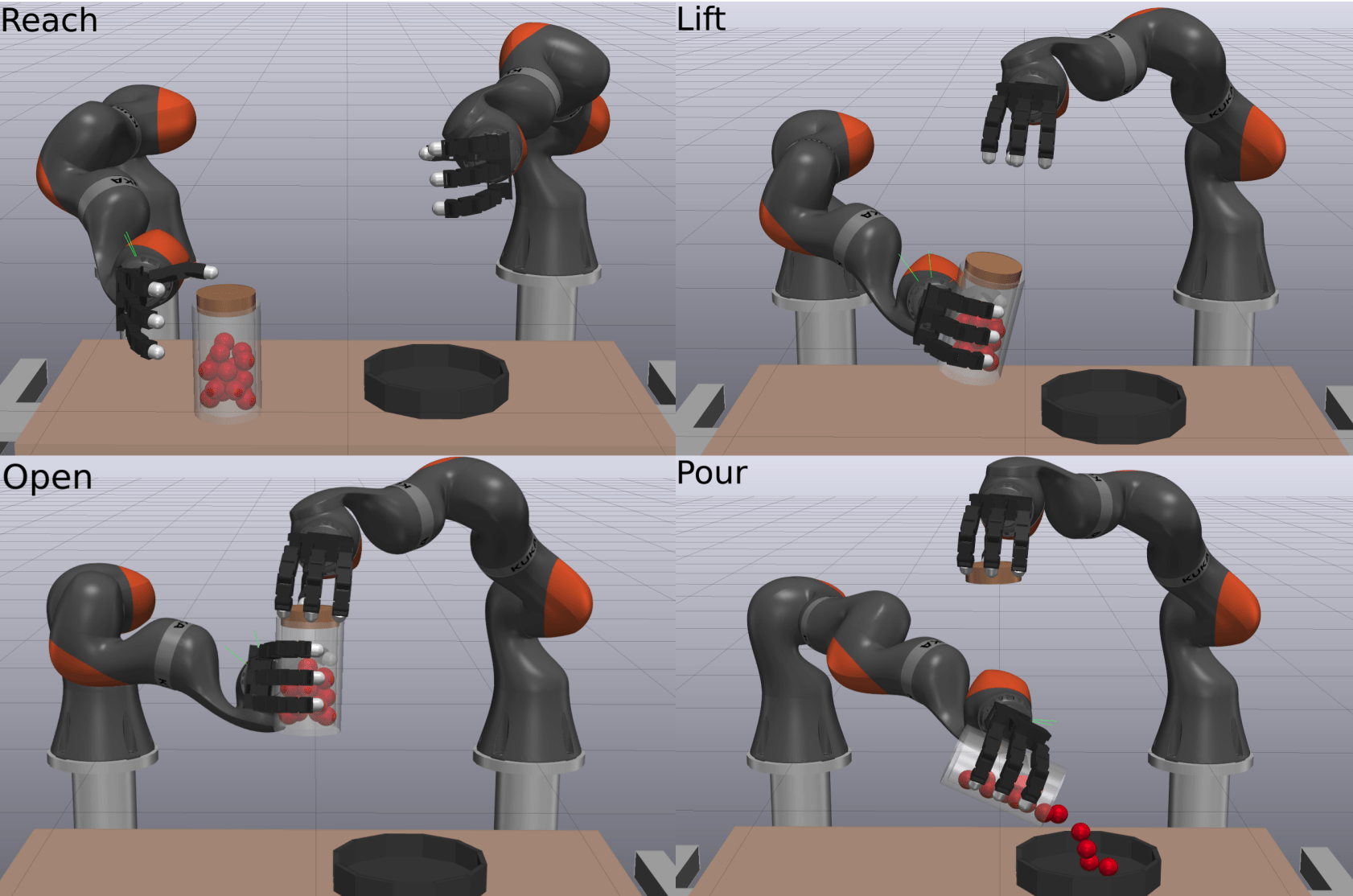
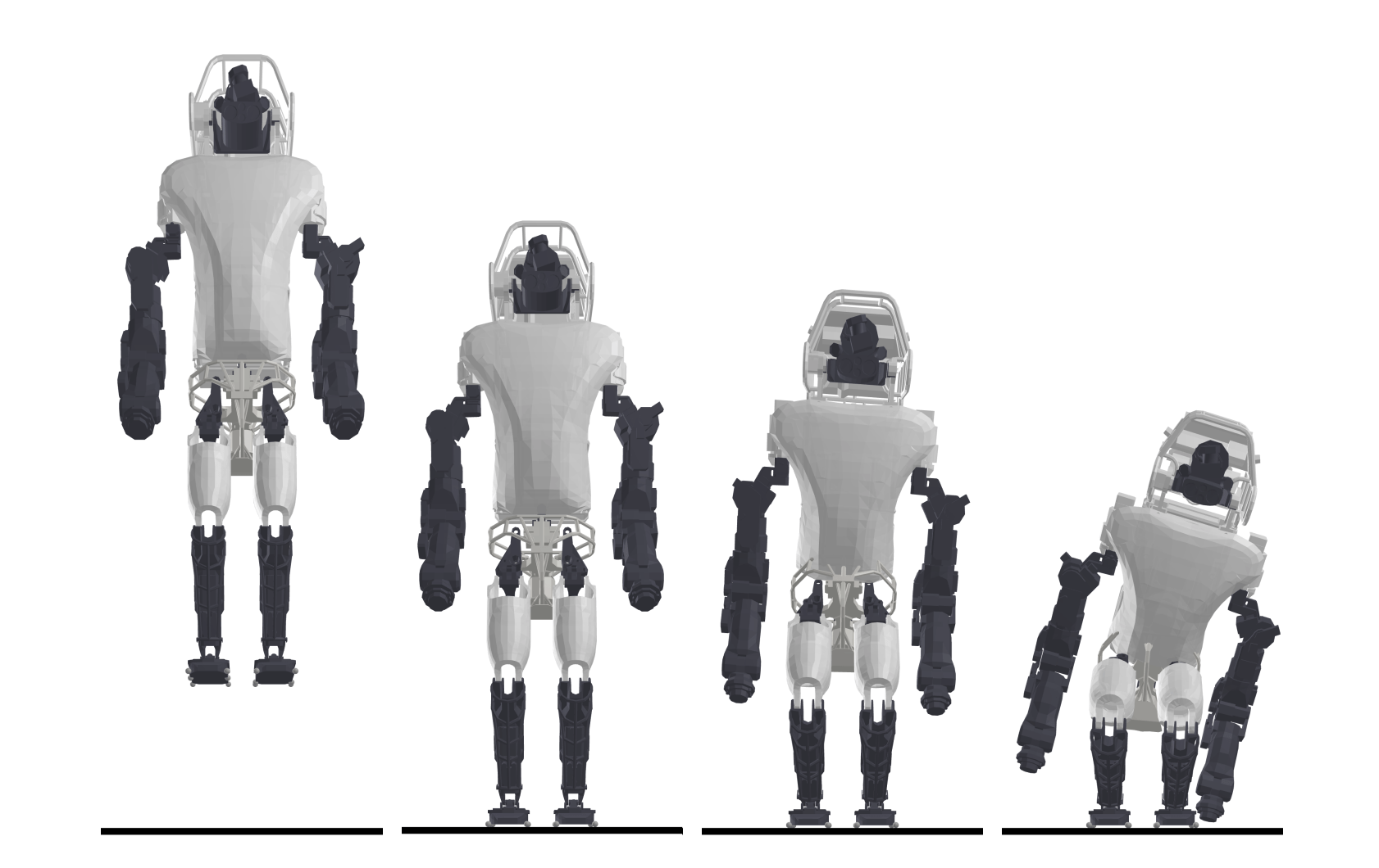
[Stewart & Trinkle, 2000]
[Mujoco, Todorov 2012]
[SAP Solver (Drake), CPH, 2022]
[Dojo, HCBKSM 2022]
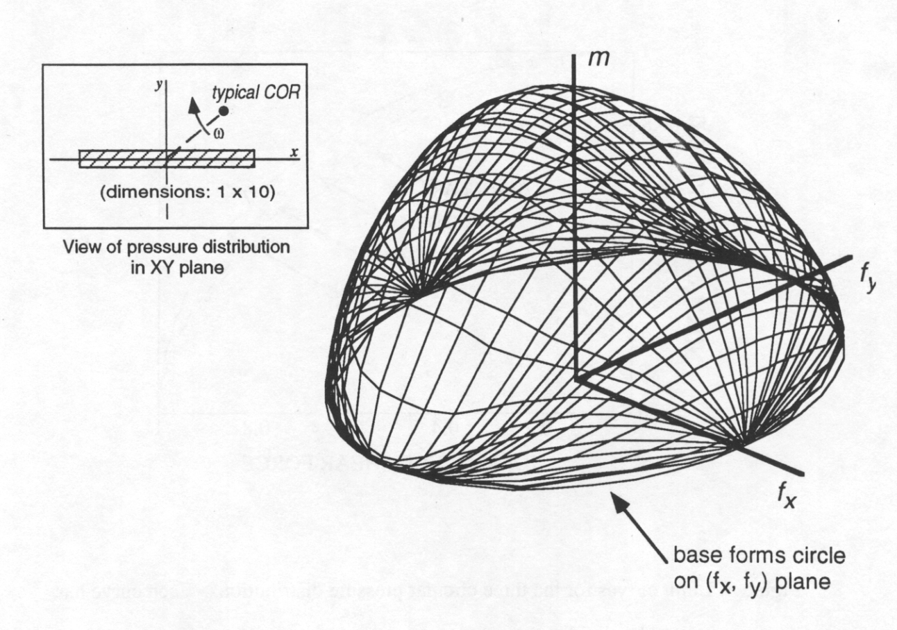
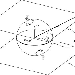
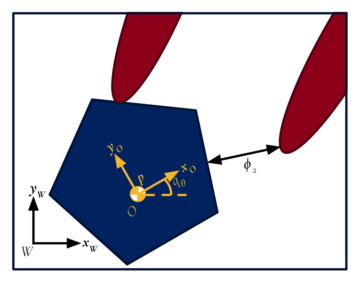
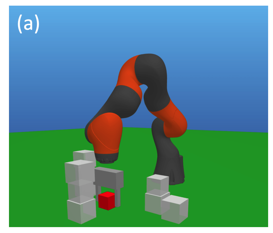
[Howe & Cutkosky 1996]
[Lynch & Mason 1996]
[Halm & Posa 2018]
[Pang & Tedrake 2021]
CQDC: A Quasi-dynamic Simulator for Manipulation

Dr. Tao Pang
Robot commands as
State only comprises of configurations
- Actuated configurations (Robot)
- Unactuated configurations (Object)
- Position command to an stiffness controller


Convex
Quasidynamic
Differentiable
Contact Model

CQDC: A Quasi-dynamic Simulator for Manipulation
CQDC: A Quasi-dynamic Simulator for Manipulation
CQDC: A Quasi-dynamic Simulator for Manipulation
Non-Penetration
Minimum Energy Principle
CQDC: A Quasi-dynamic Simulator for Manipulation
Second-Order Cone Program (SOCP)
We can use standard SOCP solvers to solve this program

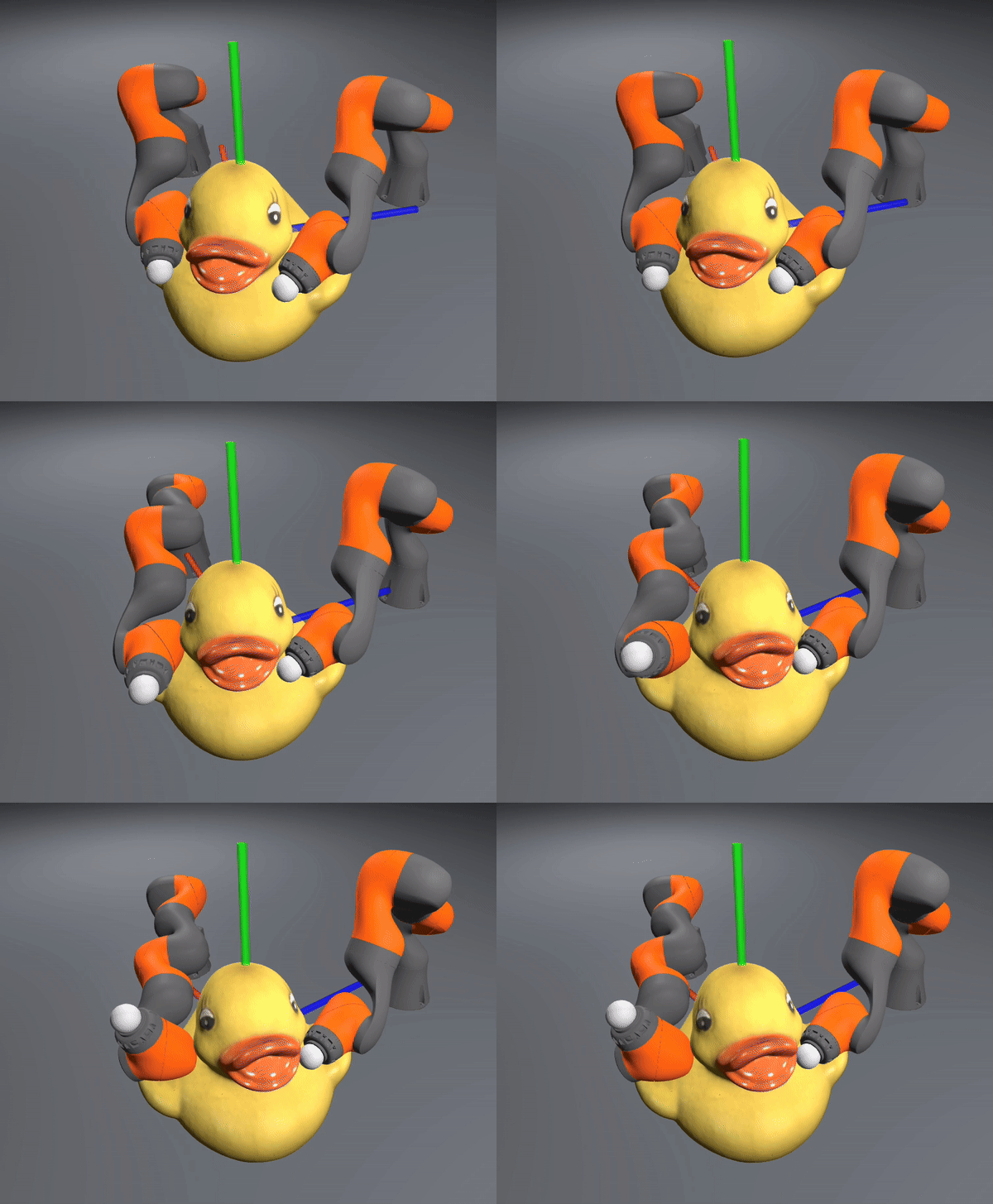
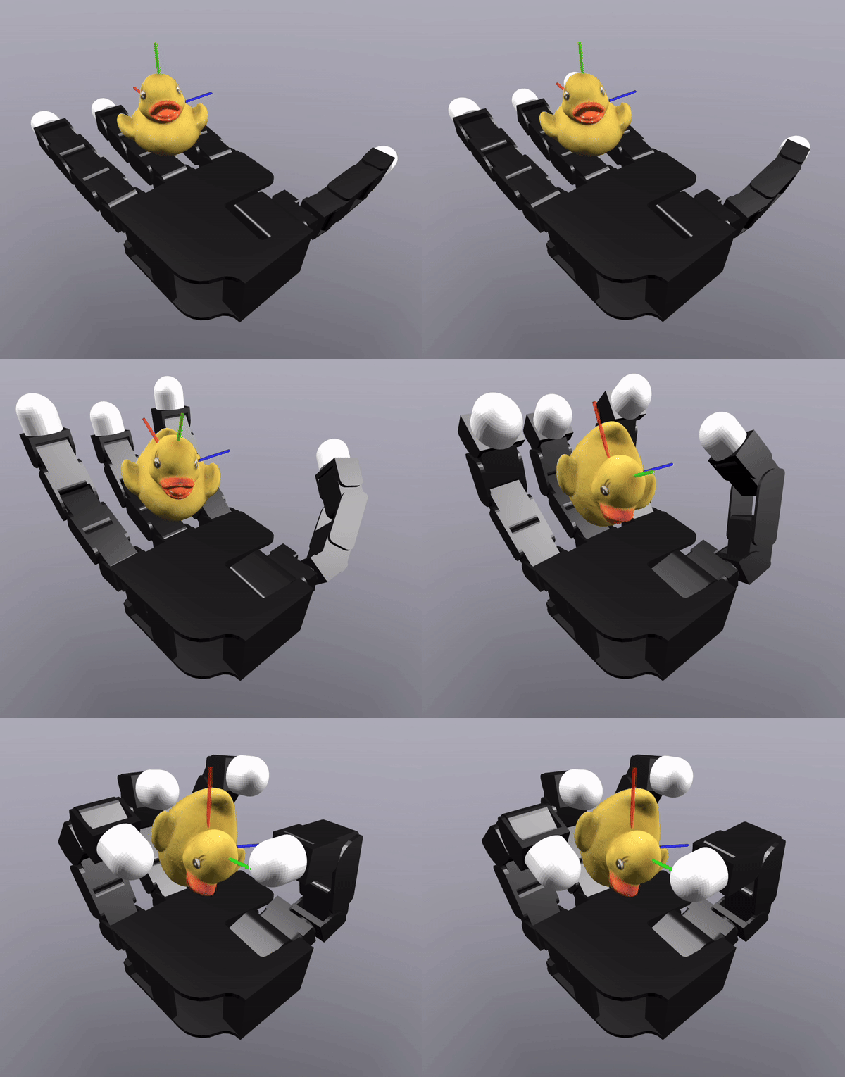
Uses Drake as Backbone

Allows us to separate complexity of "contact" from complexity of "highly dynamic".
CQDC Simulator

Sensitivity Analysis
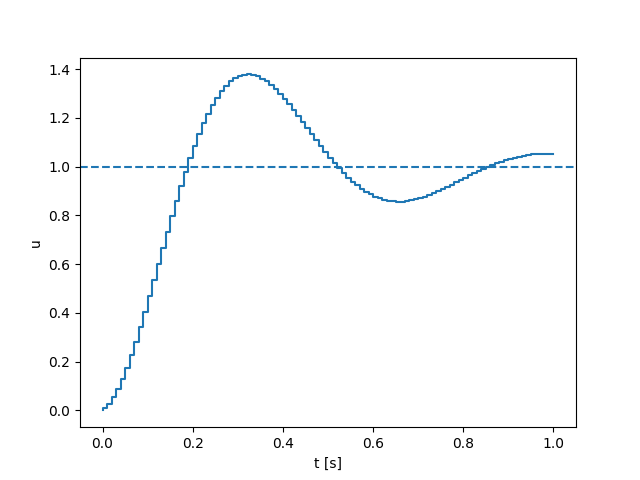
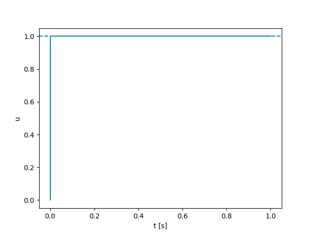
Spring-damper modeling
Quasi-static Dynamics
Directly obtained by sensitivity analysis
Jumping from one equilibrium to another lets us compute long horizon gradients temporally, allowing us to be less stiff.
Figures from Tao Pang's Defense, 2023
Constrained Optimization
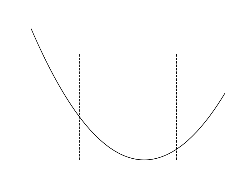
Constrained Optimization

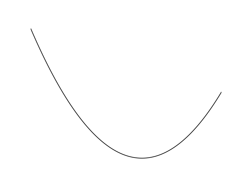
Log-Barrier Relaxation

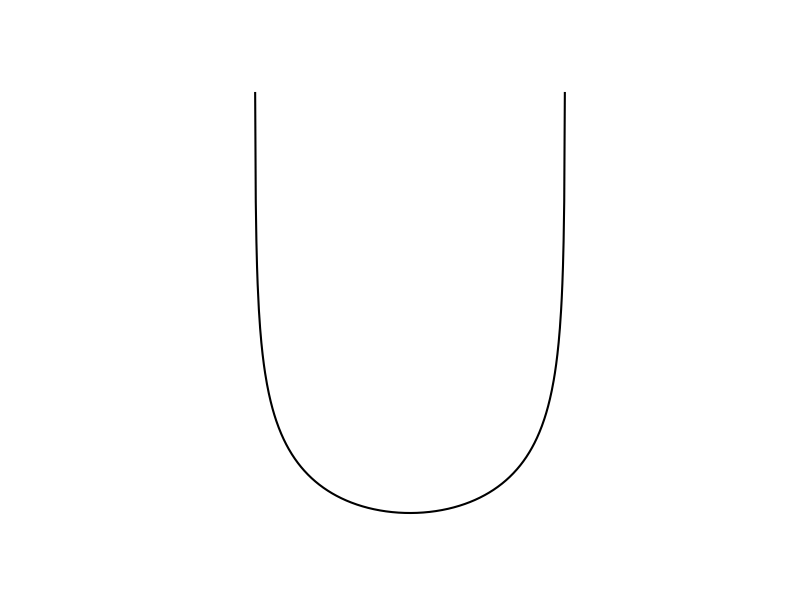


Log-Barrier Relaxation


Constraints have an inversely proportional effect to distance.
Barrier-Smoothed Dynamics
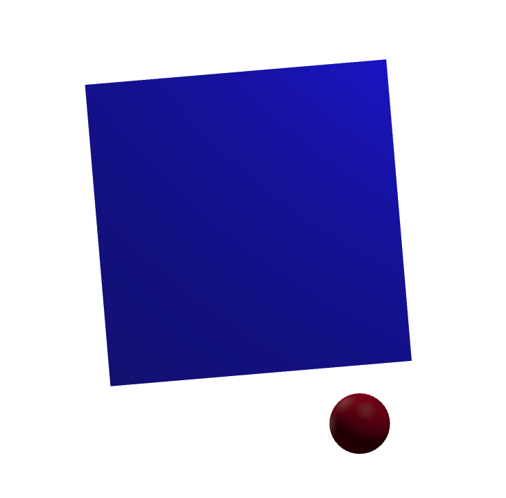
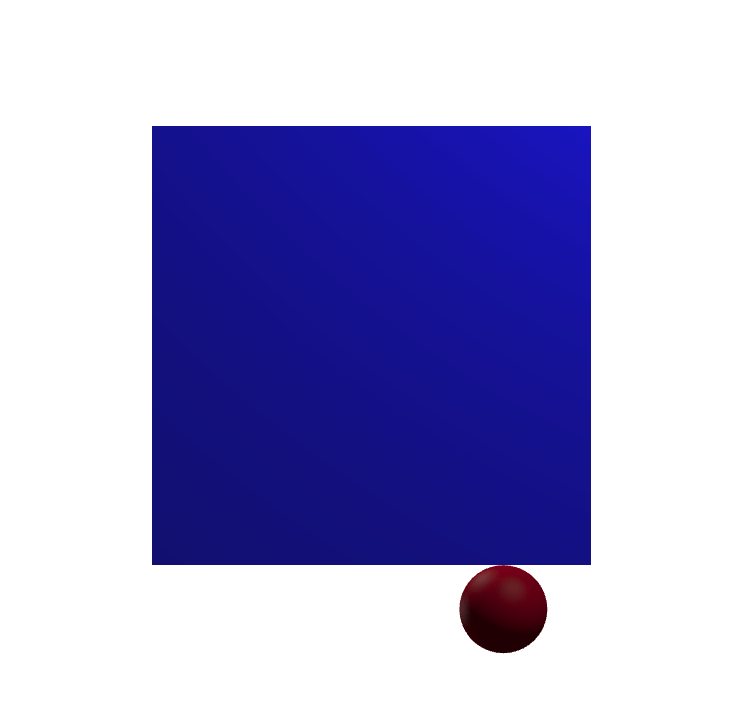
Initial Configuration
1-Step Dynamics
(Low Smoothing)
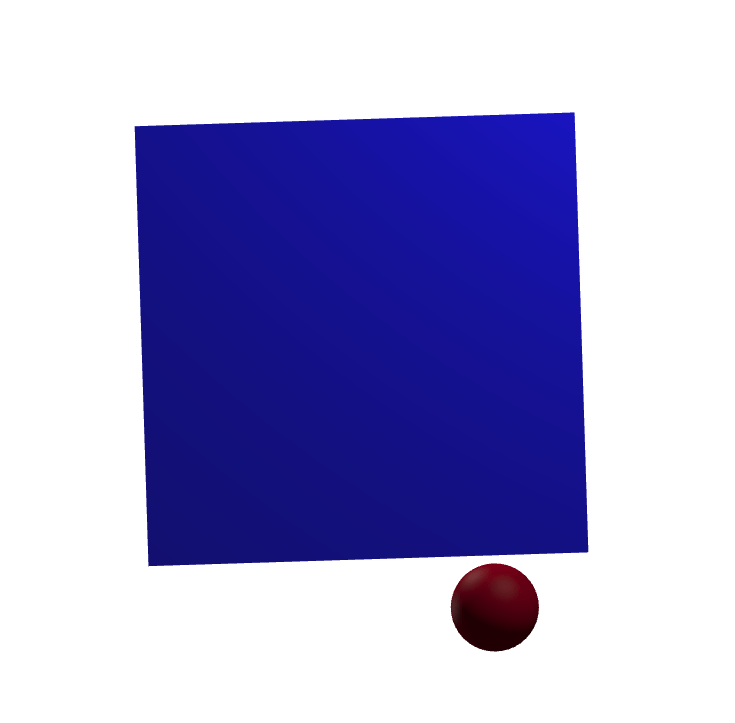
1-Step Dynamics
(High Smoothing)
Barrier smoothing creates force from a distance
Benefits of Smoothing
[ICML 2022]

Recall smoothing achieves abstraction of contact modes
Benefits of Smoothing
True Dynamics
Local Model
Benefits of Smoothing
Smoothed Dynamics
Local Model
Benefits of Smoothing
Smoothed Dynamics
Local Model
Barrier Smoothing can also abstract contact modes!
But does it have the exact same effect as randomized?
Randomized-Smoothed Dynamics
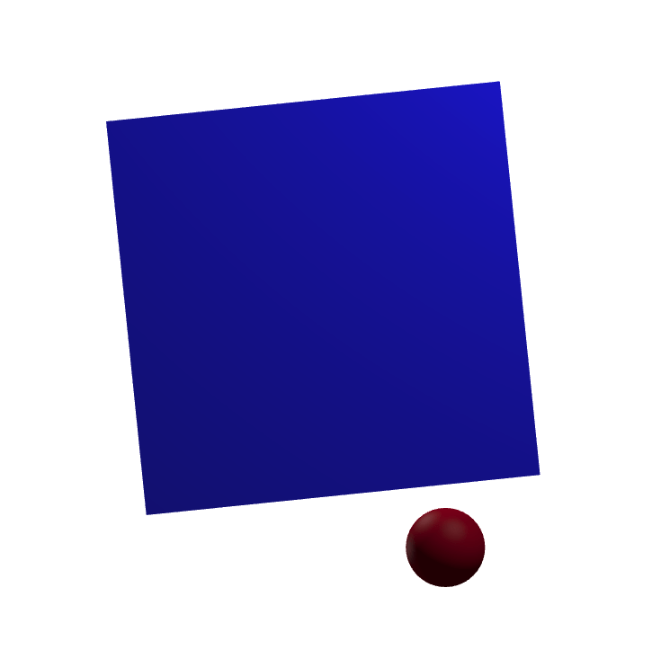

Initial Configuration
1-Step Dynamics
Sampling
Equivalence of Smoothing Schemes
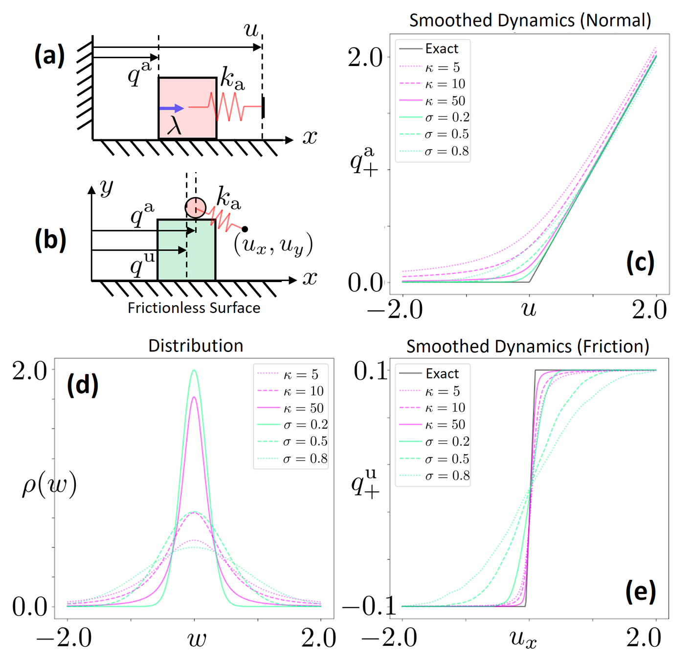
The two smoothing schemes are equivalent!
(There is a distribution that corresponds to barrier smoothing)

Randomized Smoothing

Barrier Smoothing
Analytic Expression
First-Order Gradient Estimator
Zeroth-Order Gradient Estimator
- Requires differentiability over dynamics
- Generally lower variance.
- Least requirements (blackbox)
- High variance.
Possible for only few cases
Structure
Efficiency


Comparison of Efficiency
[TRO 2023, TRO 2025]
Part 2. Local Planning / Control via Dynamic Smoothing
Can we do better by understanding dynamics structure?
How do we build effective local optimizers for contact?


Back to Dynamics
True Dynamics
How do we build a computationally tractable local model for iterative optimization?
True Dynamics
Back to Dynamics
Is this a good local model?
Local Model
First-Order Taylor Approximation

Gradients too myopic, suffers from flatness
Back to Dynamics
Local Model
Is this a good local model?

Gradients are more useful due to smoothing
First-Order Taylor Approximation
on Smoothed Dynamics
Back to Dynamics
Local Model
Is this a good local model?
First-Order Taylor Approximation
on Smoothed Dynamics

Gradients are more useful due to smoothing

Still violates some fundamental characteristics of contact!
Dynamics


What does this imply about reachable sets?
?
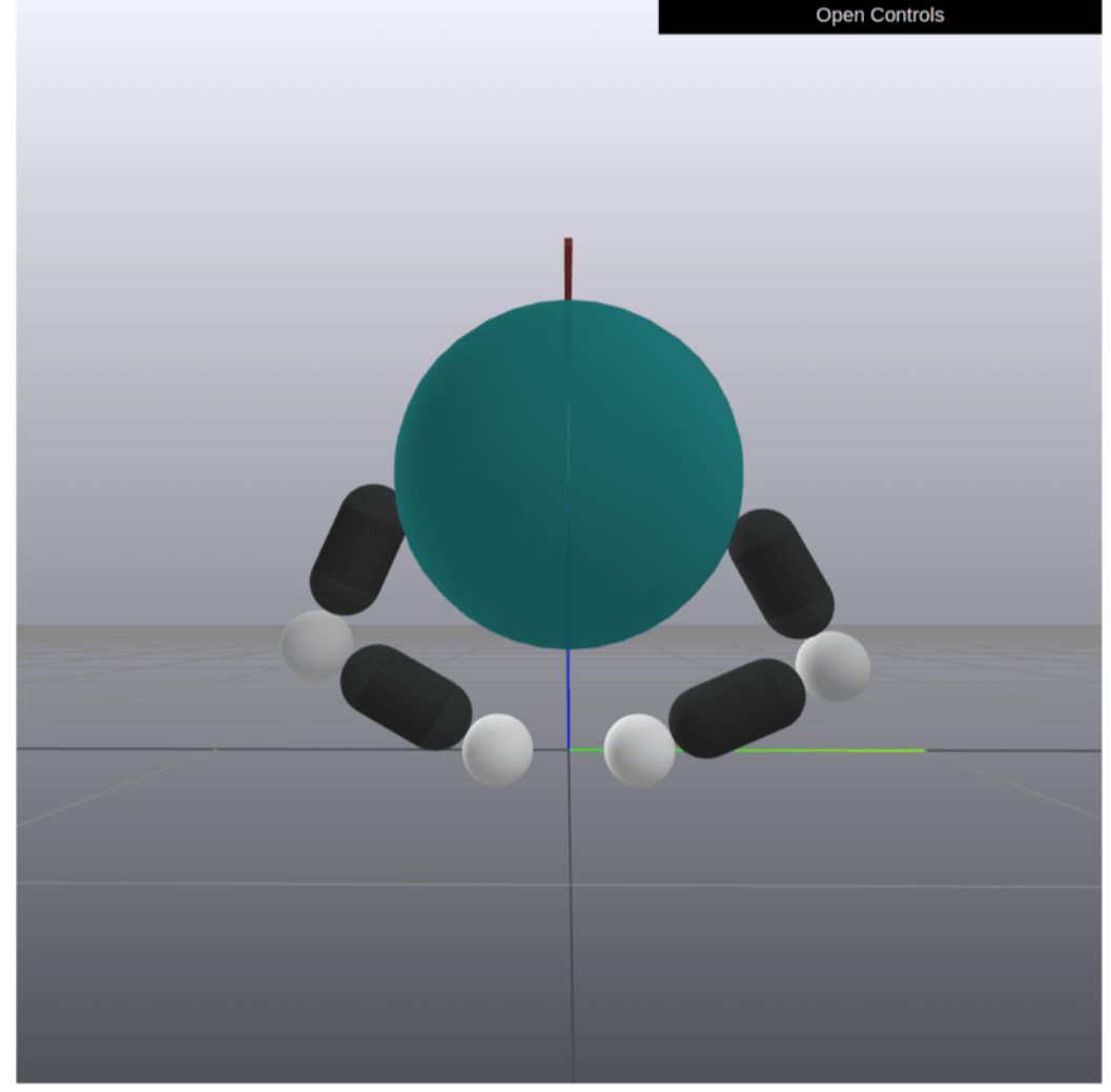
Linear Map


?
What does this imply about reachable sets?

What does this imply about reachable sets?
Linear Map


We can make ellipsoidal approximations of the reachable set

We can make ellipsoidal approximations of the reachable set

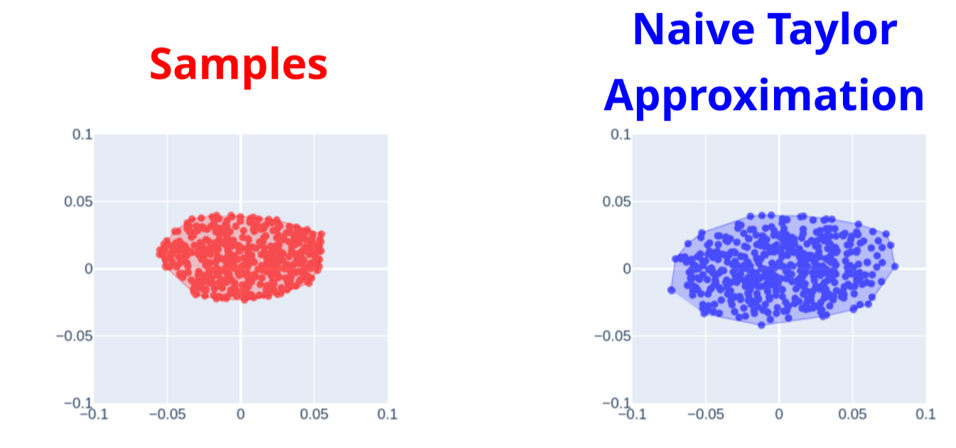
True Samples
Samples from Local Model
What does this imply about reachable sets?
Linear Map


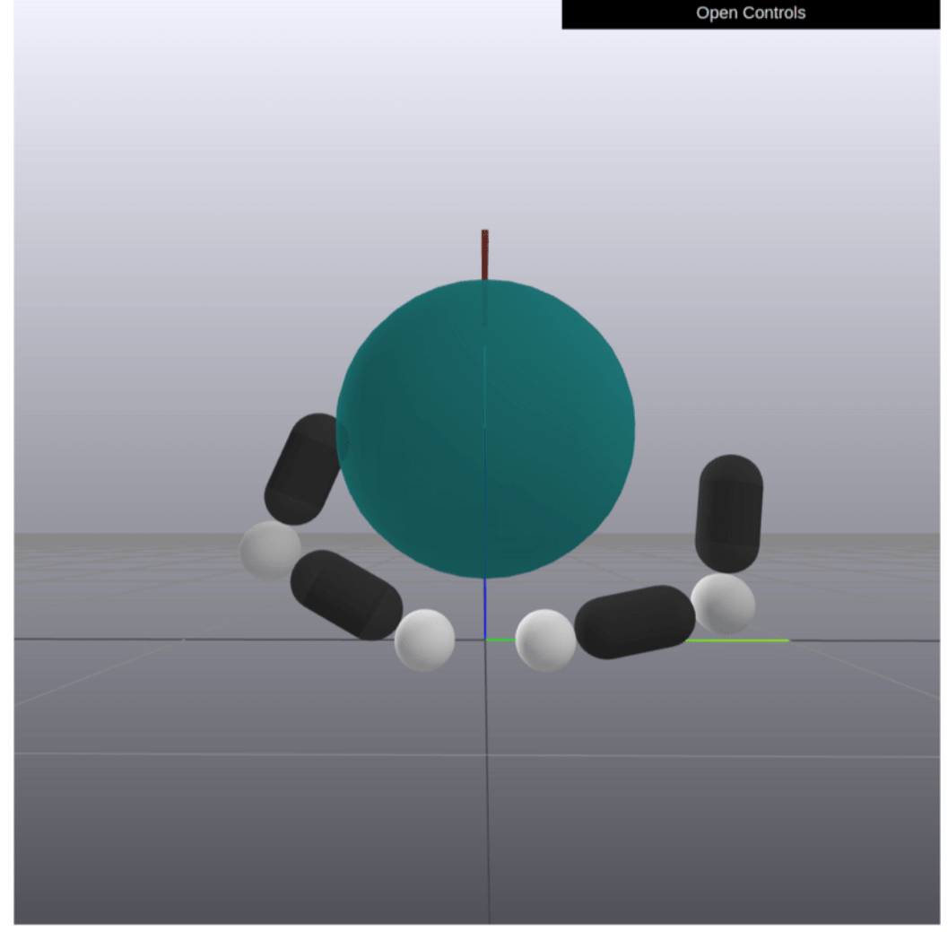
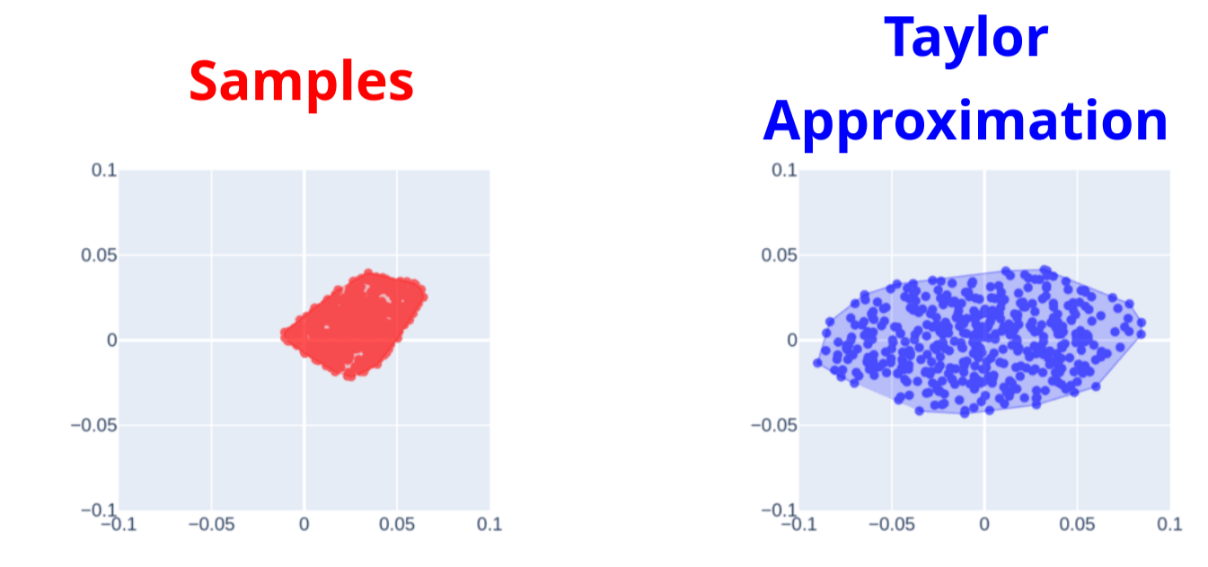
True Samples
Samples from Local Model
What does this imply about reachable sets?
Linear Map
What are we missing here?


True Samples
Samples from Local Model
What does this imply about reachable sets?
Linear Map
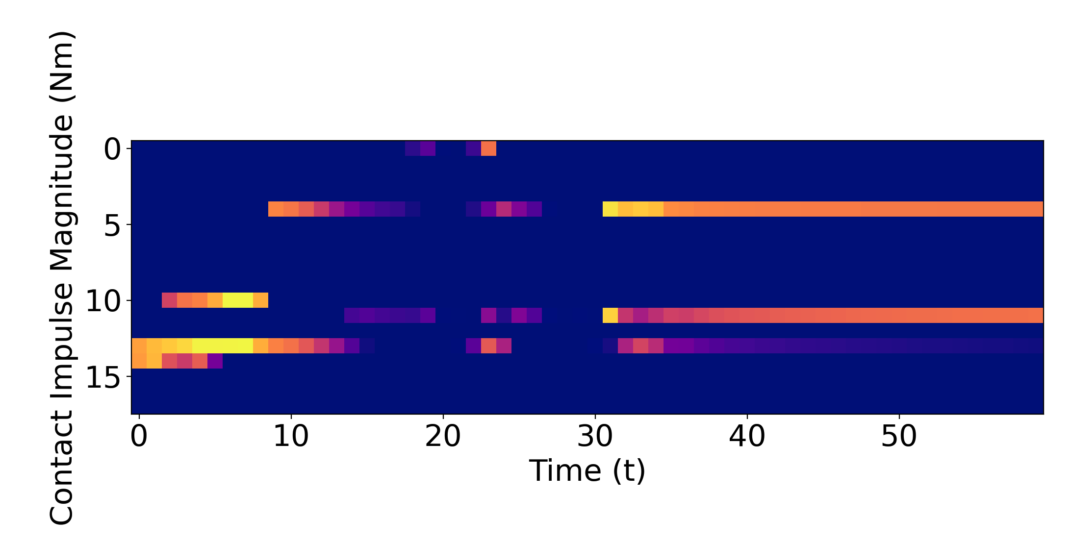
Qualification on Contact Impulses
Dynamics (Primal)


Contact Impulses (Dual)


The Friction Cone

*image taken from Stephane Caron's blog
Unilateral
(Can't pull)
Coulomb Friction
Friction Cone
+
=
Qualification on Contact Impulses
Dynamics (Primal)


Contact Impulses (Dual)


+
*image taken from Stephane Caron's blog
Contact is unilateral
Feasible Trust Region
Dynamics (Primal)
Contact Impulses (Dual)
Trust Region Size
Feasible Trust Region
Motion Set
Feasible Trust Region


Motion Set

Dynamics (Primal)
Contact Impulses (Dual)
Trust Region Size
Contact Impulse Set
Feasible Trust Region

Contact Impulse Set

Dynamics (Primal)
Contact Impulses (Dual)
Trust Region Size
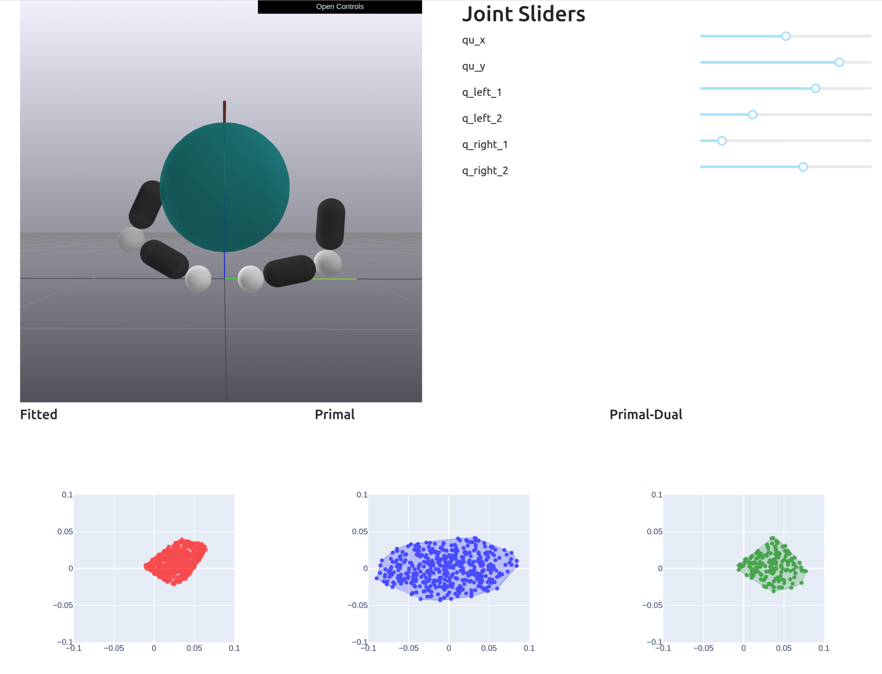
Now we have a close match with real samples
Motion Set
No Constraints
True Samples
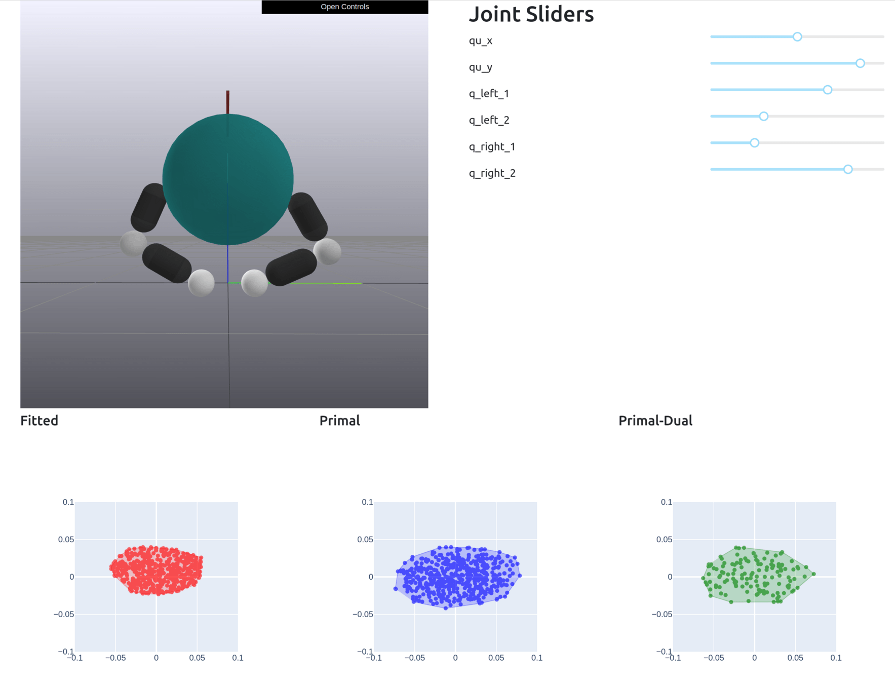
Motion Set
No Constraints
True Samples
Closer to ellipse when there is a full grasp

The gradients take into account manipulator singularities
Motion Set
No Constraints
True Samples
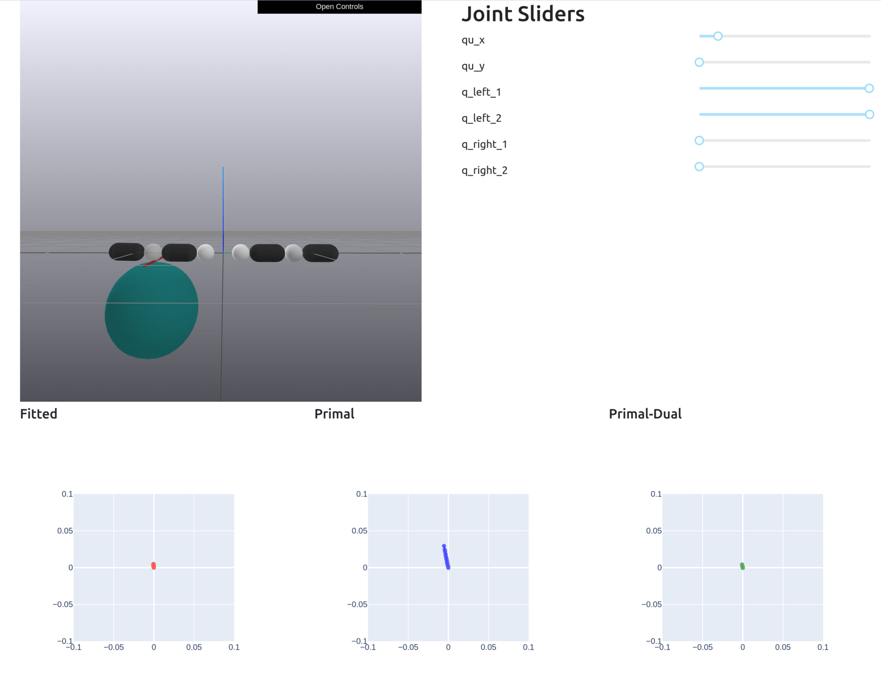
Motion Set
No Constraints
True Samples
Can also add additional convex constraints (e.g. joint limits)
Finding Optimal Action: One Step
Get to the goal
Minimize effort
Motion Set Constraint
Get to the goal
Minimize effort
Multi-Horizon Optimization
Motion Set Constraint
Trajectory Optimization: Step 1
Roll out an input trajectory guess to obtain an initial trajectory.
Trajectory Optimization: Step 2
Linearize around each point to obtain a local dynamics model around the trajectory
Trajectory Optimization: Step 3
Use our subproblem to solve for a new input trajectory
Trajectory Optimization: Iteration
Roll out the new input trajectory guess and repeat til convergence
Model Predictive Control (MPC)
Plan a trajectory towards the goal in an open-loop manner
Model Predictive Control (MPC)
Execute the first action.
Due to model mismatch, there will be differences in where we end up.
Model Predictive Control (MPC)
Replan from the observed state,
execute the first action,
and repeat.
MPC Rollouts

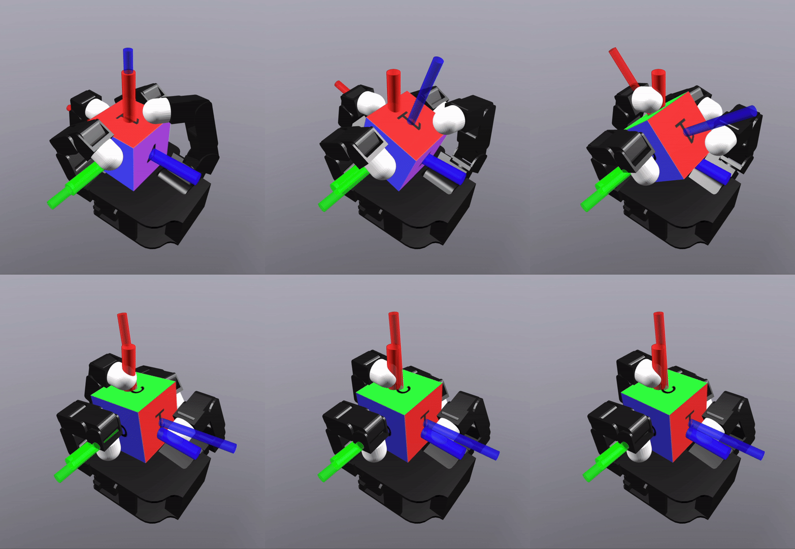
Able to stabilize to plan to the goal in a contact-rich manner
MPC Rollouts
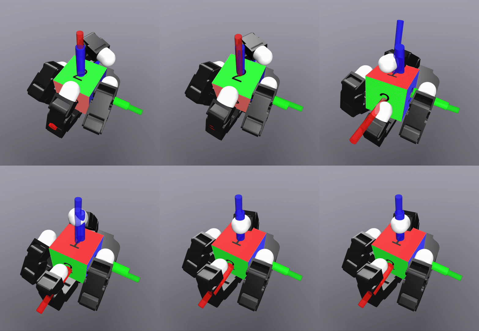

The controller also successfully scales to the complexity of dexterous hands
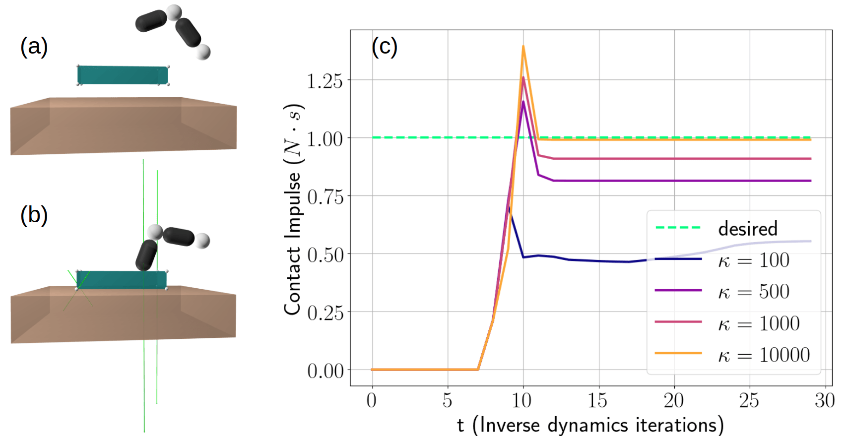
Force Control
Having a model of contact impulses allows us to perform force control
Applied desired forces
Minimize effort
Contact Impulse Set
Force Control
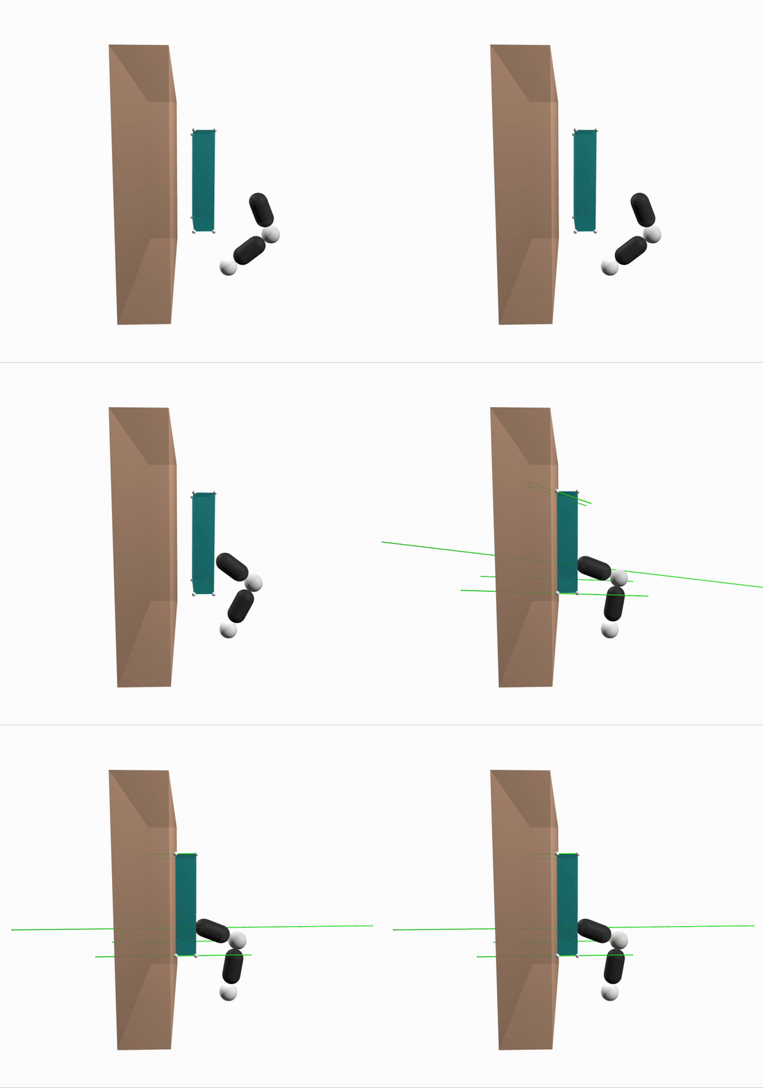
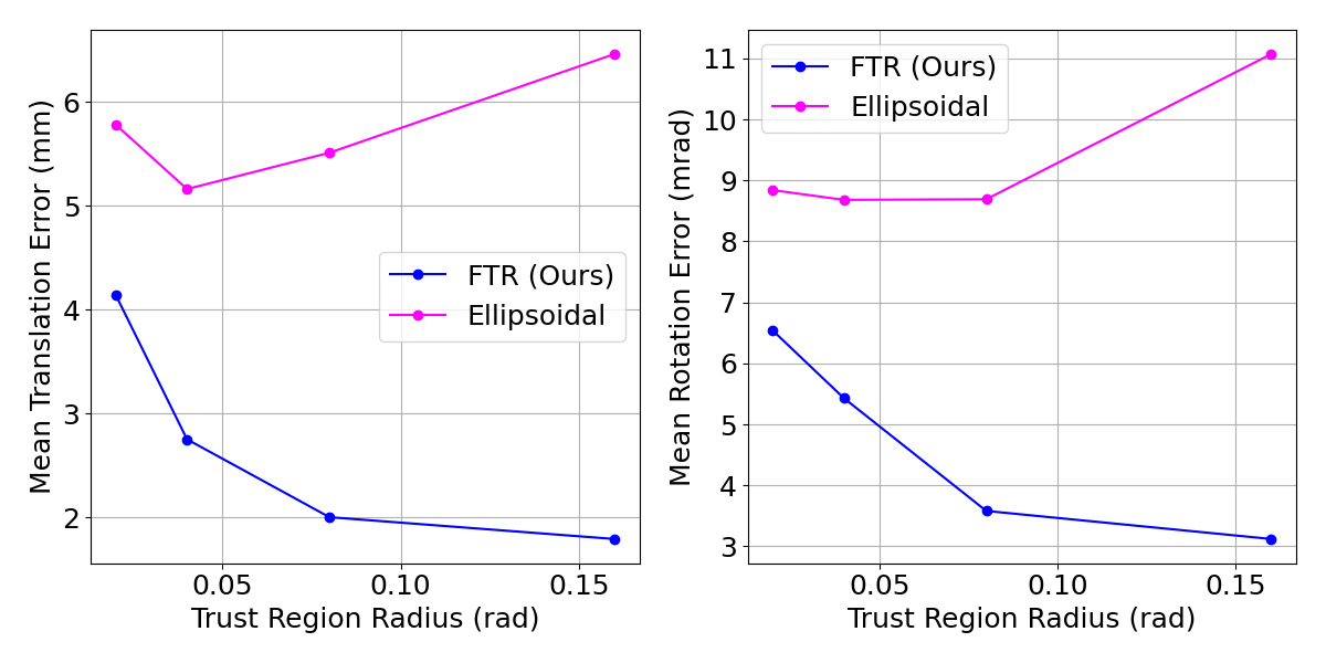
Is the friction cone constraint necessary?
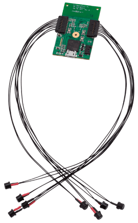
Hardware Setup
Small IR LEDs which allow motion capture & state estimation
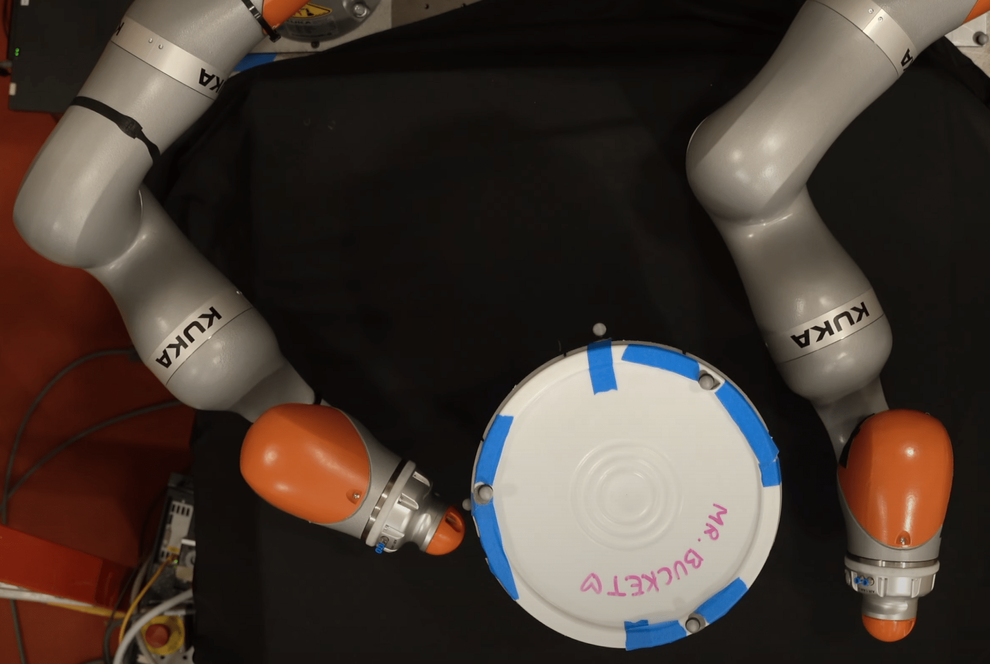
iiwa bimanual bucket rotation
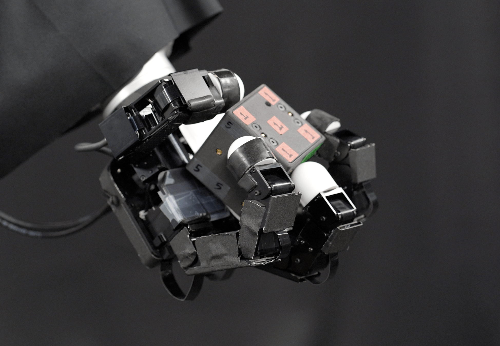
allegro hand in-hand reorientation
Mocap markers
[TRO 2023, TRO 2025]
Part 2. Local Planning / Control via Dynamic Smoothing
Can we do better by understanding dynamics structure?
How do we build effective local optimizers for contact?


[TRO 2023, TRO 2025]
Part 3. Global Planning for Contact-Rich Manipulation
Part 2. Local Planning / Control via Dynamic Smoothing
Part 1. Understanding RL with Randomized Smoothing

Introduction

[TRO 2023, TRO 2025]
Part 3. Global Planning for Contact-Rich Manipulation
What are fundamental limits of local control?
How can we address difficult exploration problems?
How do we achieve better global planning?
Reduction to Motion Planning over Smooth Systems

Smoothing lets us...
- Abstract contact modes
- Gets rid of discreteness coming from granular contact modes.
Contact-Rich Manipulation
Motion Planning over Smooth Systems
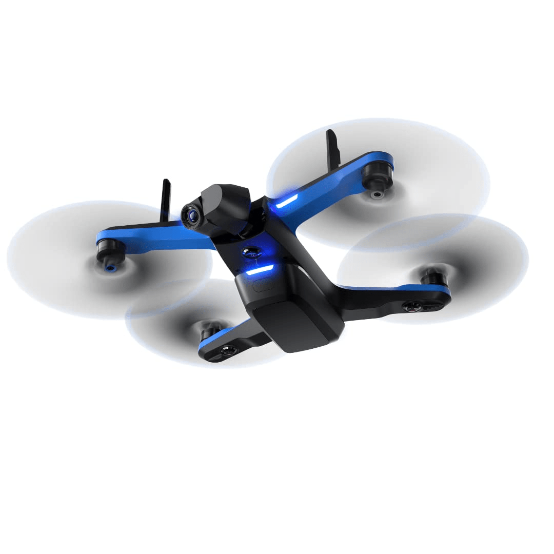

Discreteness of Motion Planning


Discreteness of Motion Planning


Discreteness of Motion Planning


Discreteness of Motion Planning


Discreteness of Motion Planning


Discreteness of Motion Planning
Discreteness of Motion Planning


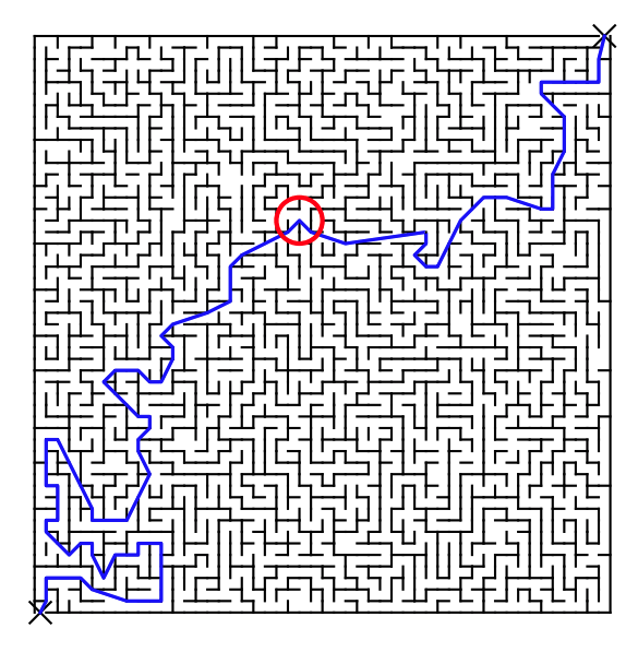
Marcucci et al., 2022
Motion Planning over Smooth Systems is not necessarily easier
The Exploration Problem
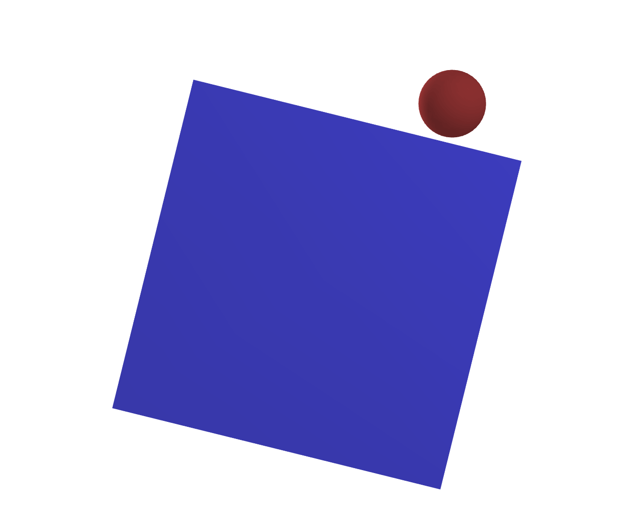
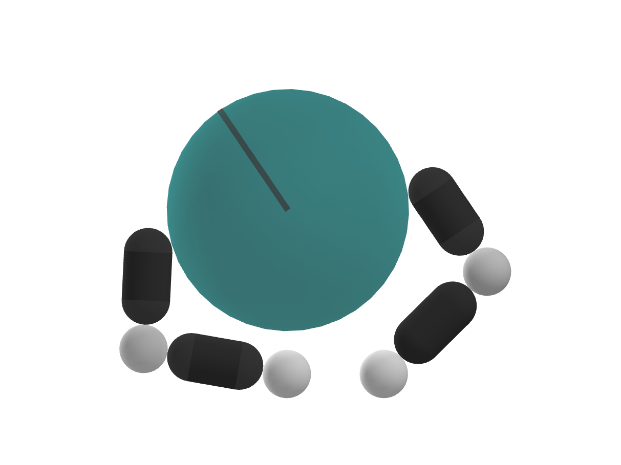

How do we push in this direction?
How do we rotate further in presence of joint limits?

How do we push in this direction?
The Exploration Problem
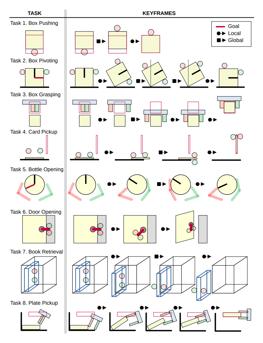
The Exploration Problem

How do I know that I need to open my finger to grasp the box?
[TRO 2023, TRO 2025]
Part 3. Global Planning for Contact-Rich Manipulation
What are fundamental limits of local control?
How can we address difficult exploration problems?
How do we achieve better global planning?


The Exploration Problem

Because I have seen that this state is useful!
Local Control


What is a sequence of actions I must take to push the box down?
Local Search for Open-Loop Actions
The Reset Action Space


What is a sequence of actions I must take to push the box down?

Where should I place my finger if I want to make progress towards the goal?
Local Search for Open-Loop Actions
Global Search for Initial Configurations
The Reset Action Space
Utilizing the MPC Cost
Our Local Controller
How well does the policy perform when this controller is run closed-loop?

Get to the goal
Minimize effort
Motion Set Constraint
The Actuator Relocation Problem
Choose best initial actuator configuration for MPC
Non-penetration constraints
Where should I place my finger if I want to make progress towards the goal?
Global Search for Initial Configurations
Robustness Considerations
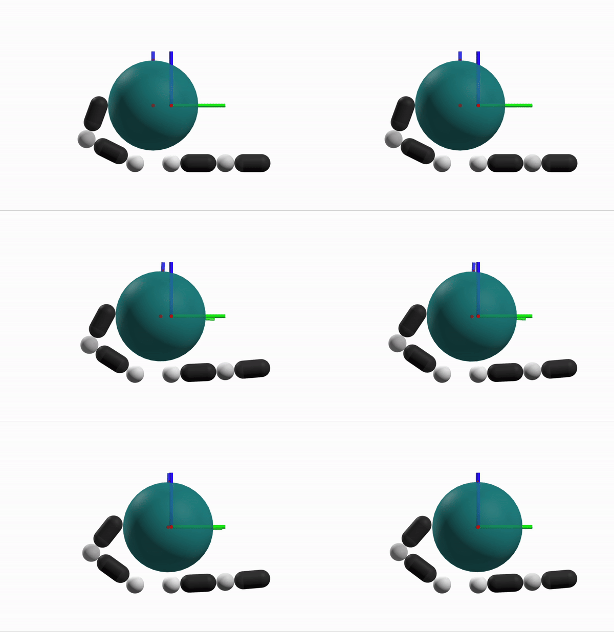
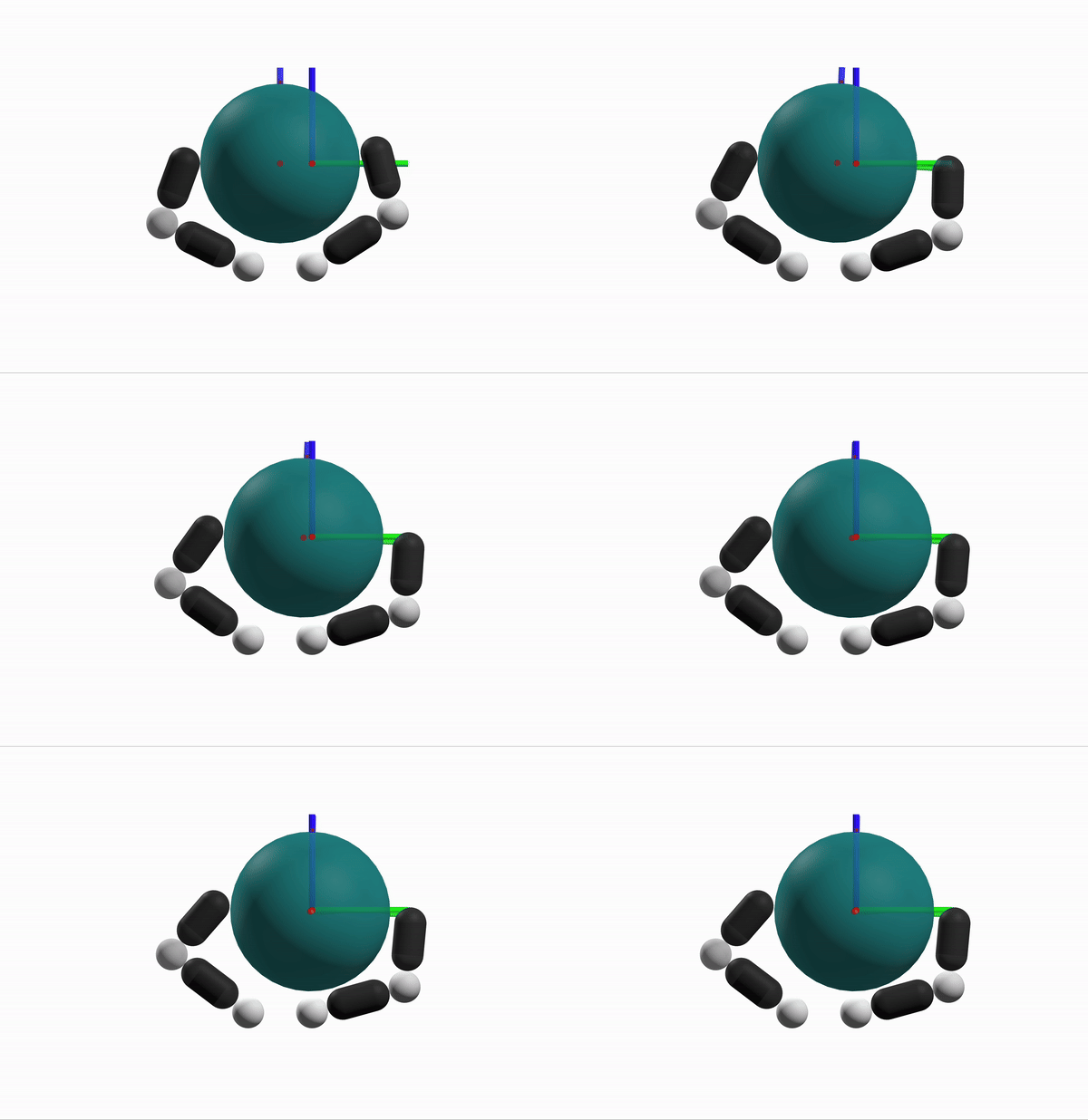
What is a better configuration to start from?
Robustness Considerations
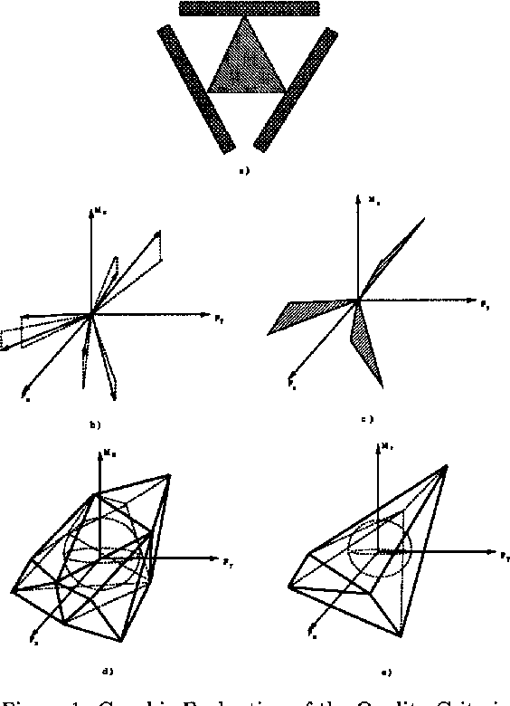
[Ferrari & Canny, 1992]


We prefer configurations that can better reject disturbances
Regularizing with Robustness
How do we efficiently find an answer to this problem?
The Actuator Relocation Problem
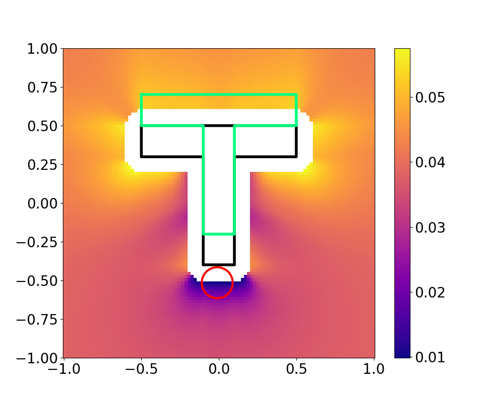
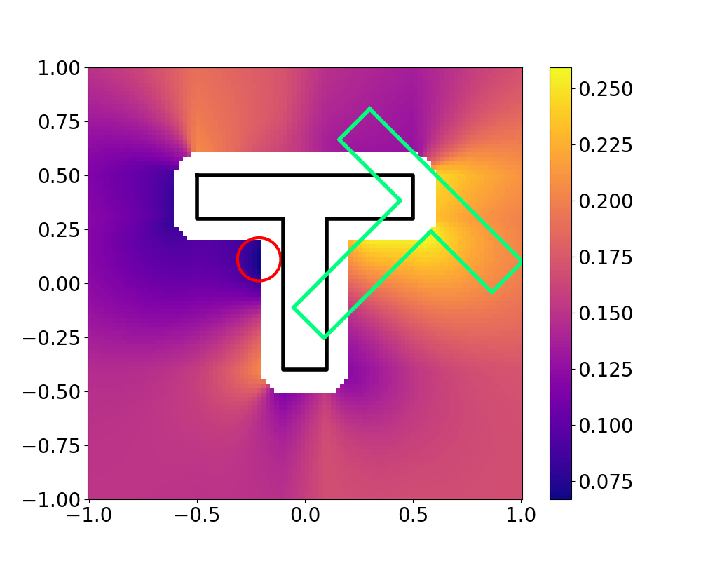
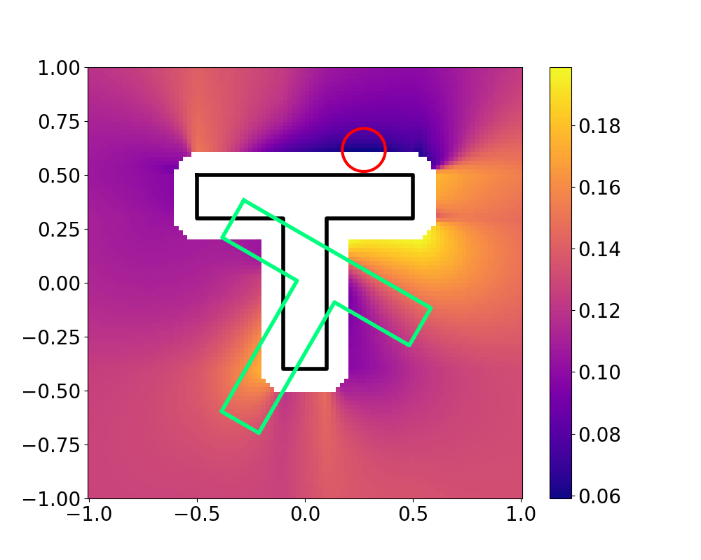
Landscape of the value function is much more complex,
so we resort to sampling-based search
Grasp Synthesis Procedure
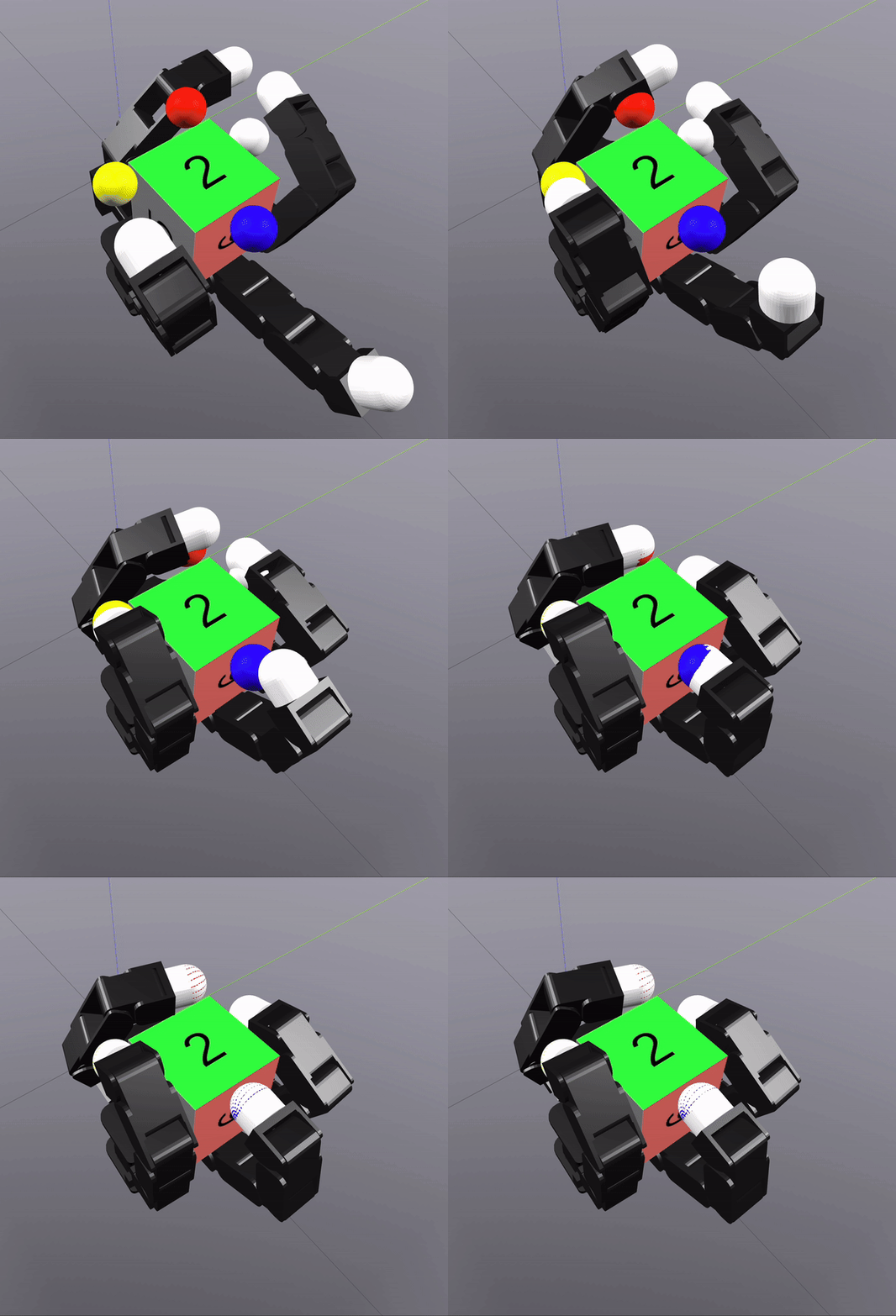
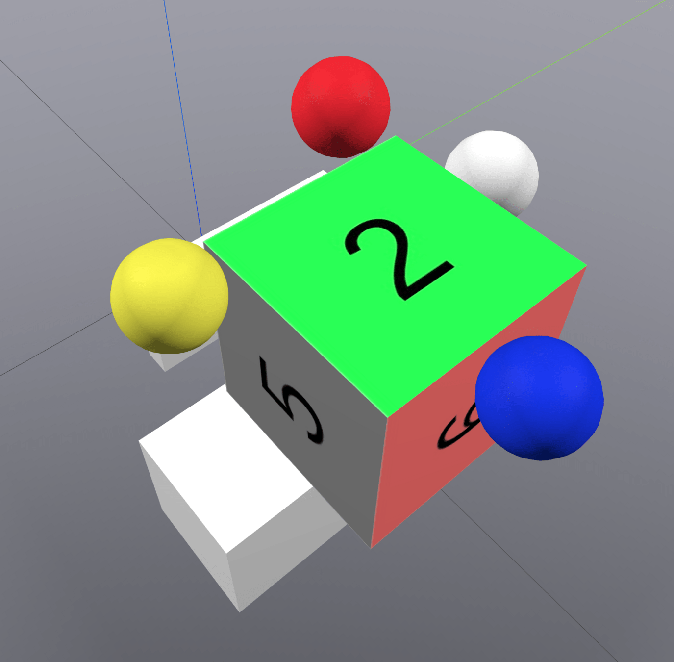
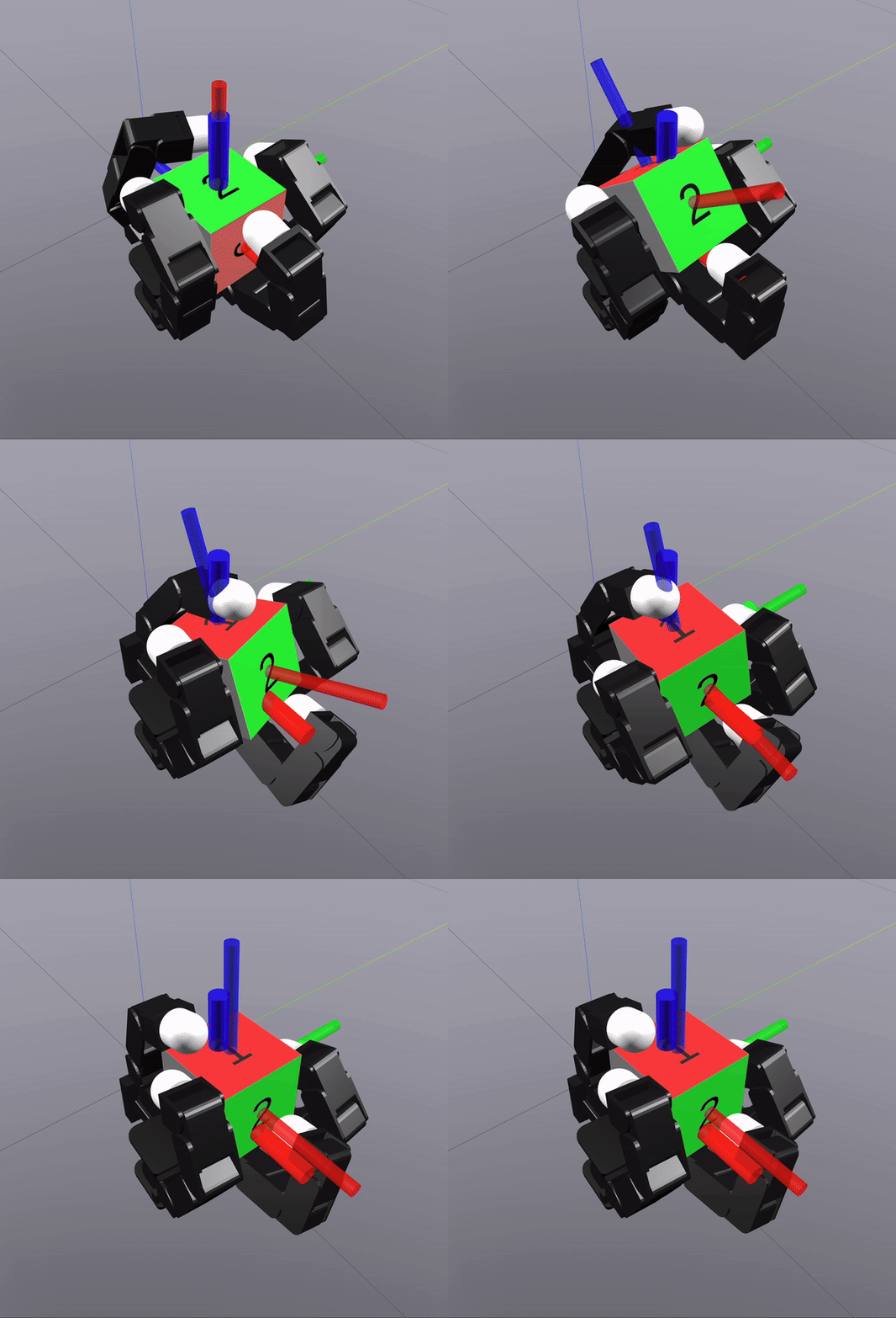
Sampling-Based Search on
Reduced-Order System
Differential Inverse Kinematics to find Hand Configuration
Verification with MPC rollouts
Grasp Synthesis Results


Pitch + 90 degrees
Yaw + 45 degrees
Pitch - 90 degrees
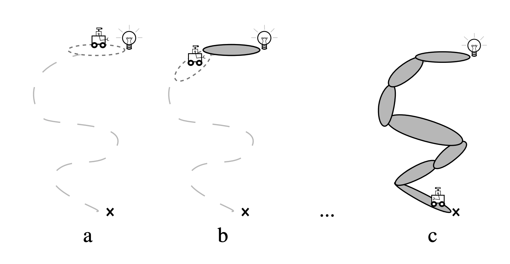
Konidaris & Barto,
Skill Chaining (2009)
Primitive View on Grasp Synthesis + MPC
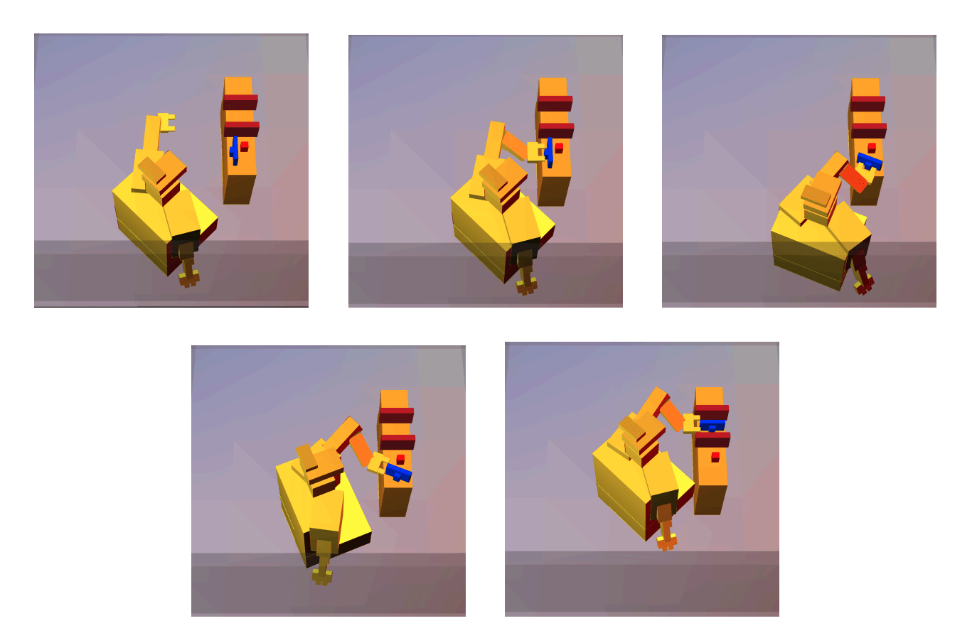
TLP & LPK (2014)
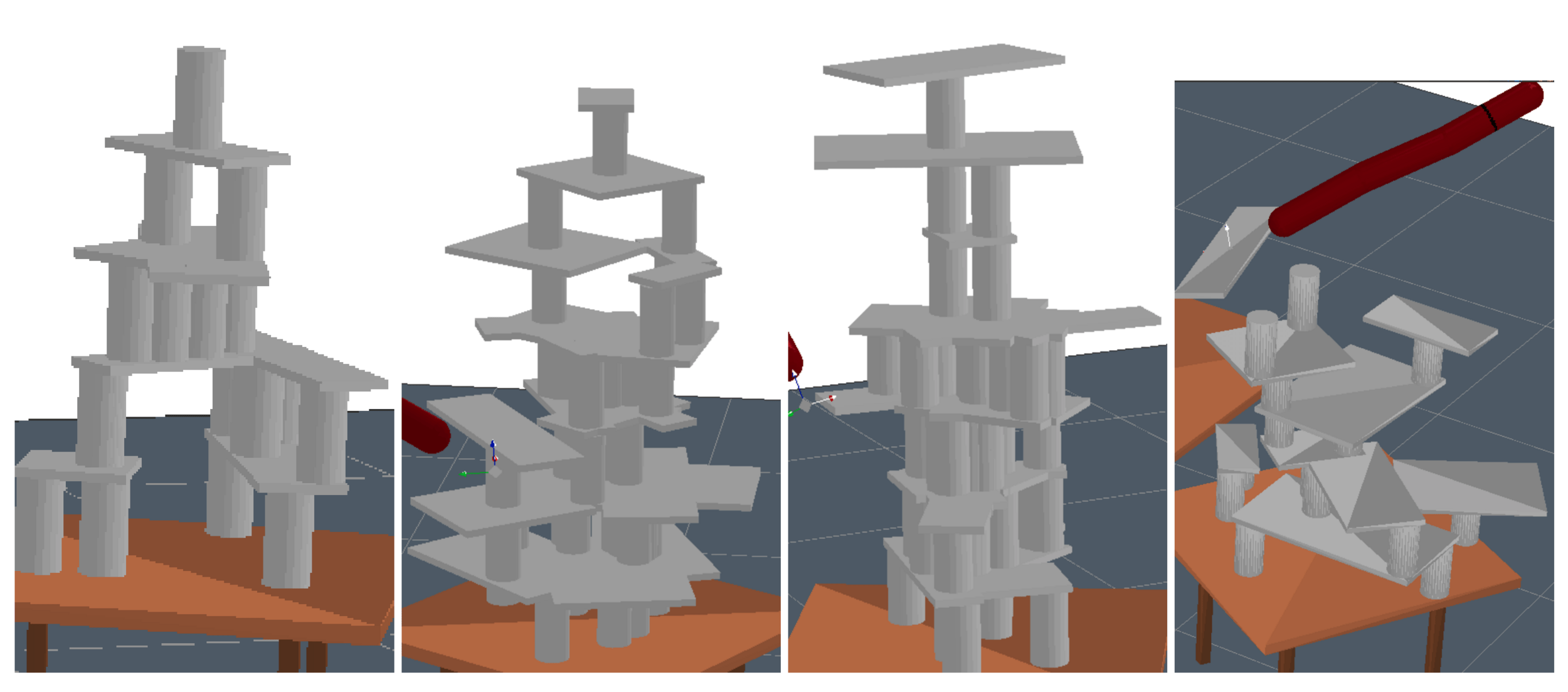
Toussaint
Logic-Geometric Programming (2015)
We have introduced discreteness by defining a primitive
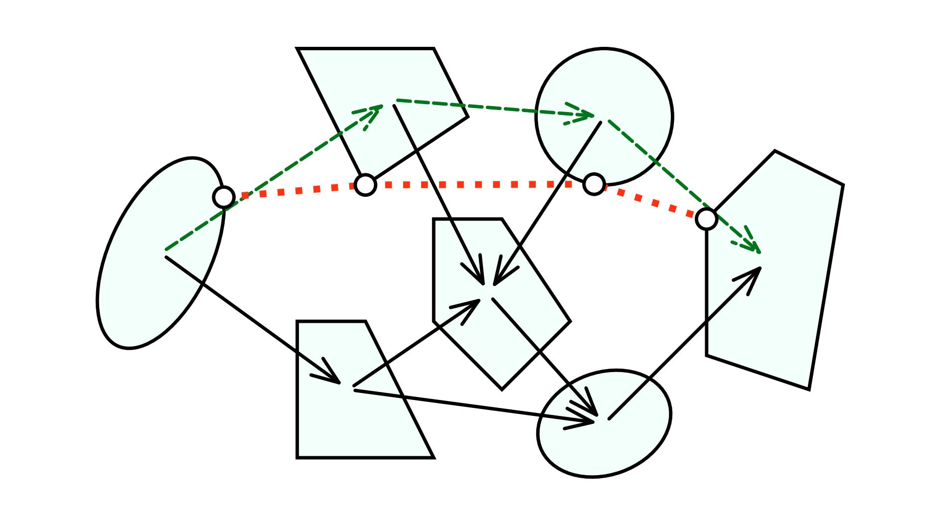
TM & JU & PP & RT
Graph of Convex Sets (2023)
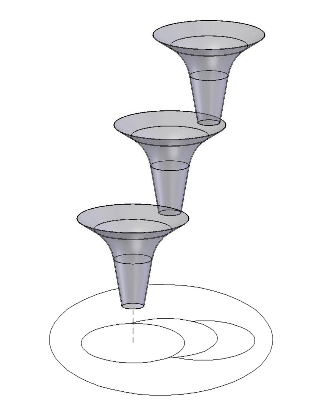
Tedrake,
LQR-Trees (2009)
[TRO 2023, TRO 2025]
Part 3. Global Planning for Contact-Rich Manipulation
What are fundamental limits of local control?
How can we address difficult exploration problems?
How do we achieve better global planning?


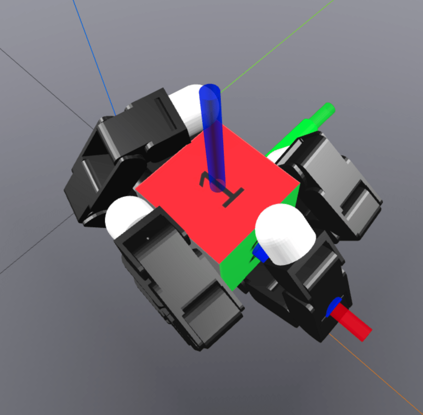
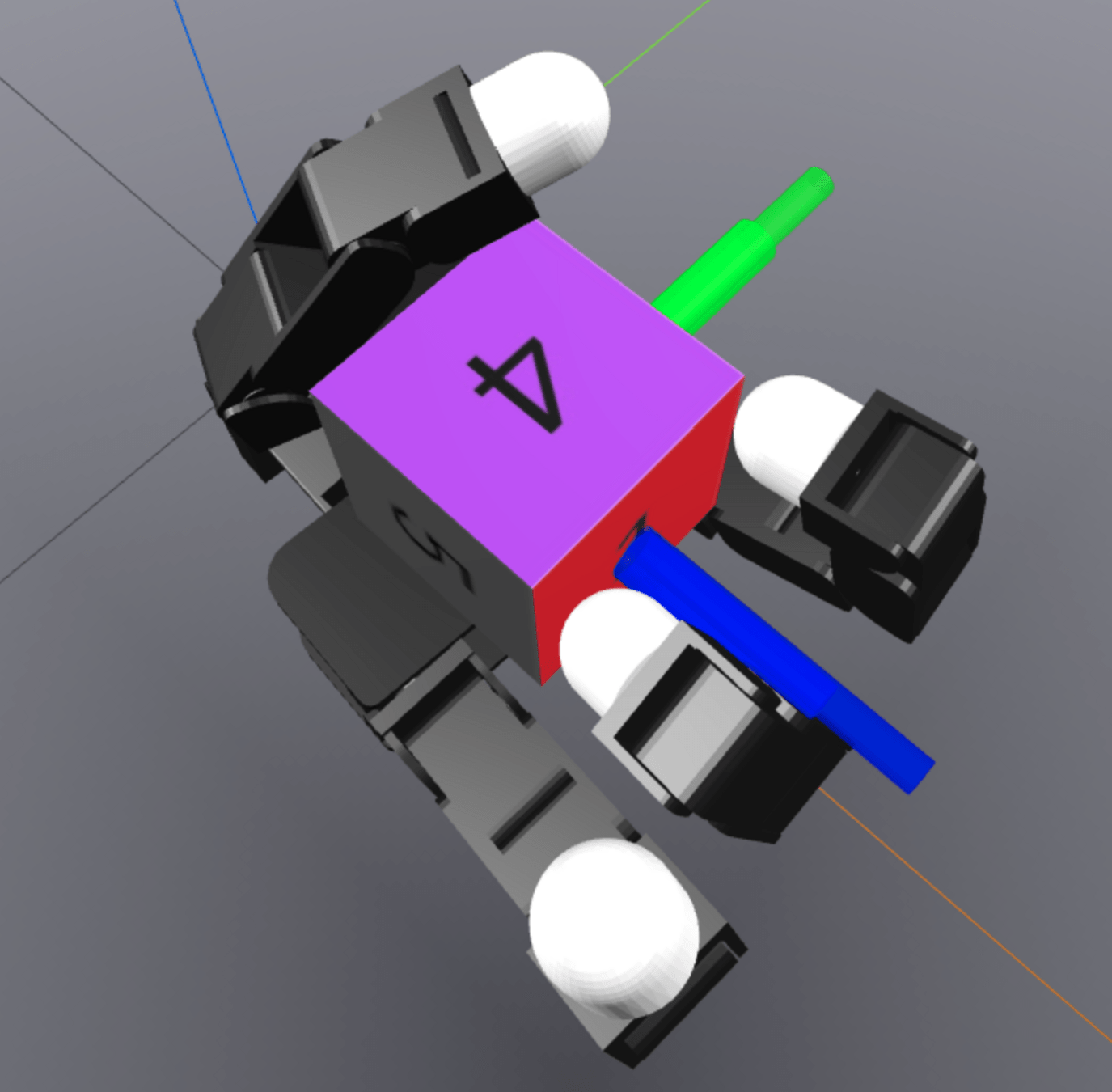
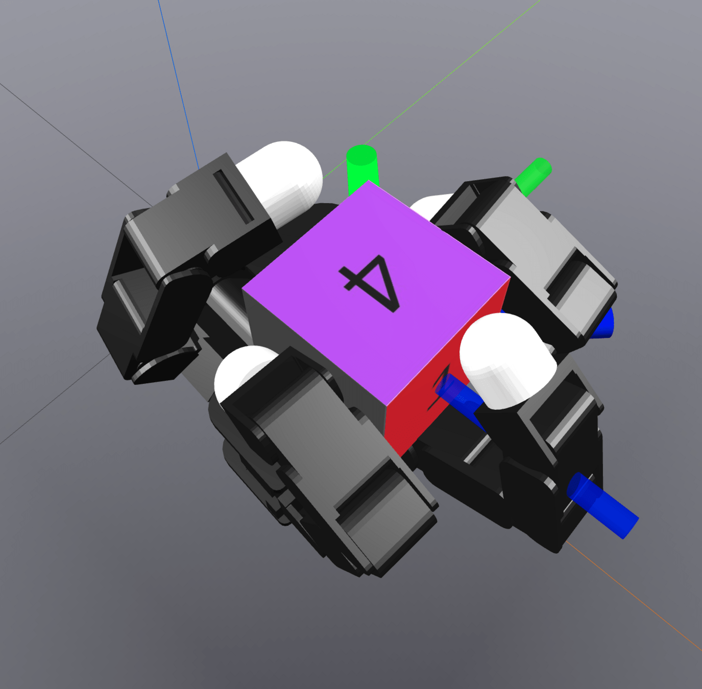
Chaining Local Actions
MPC
MPC
Regrasp
(Collision-Free Motion Planning)
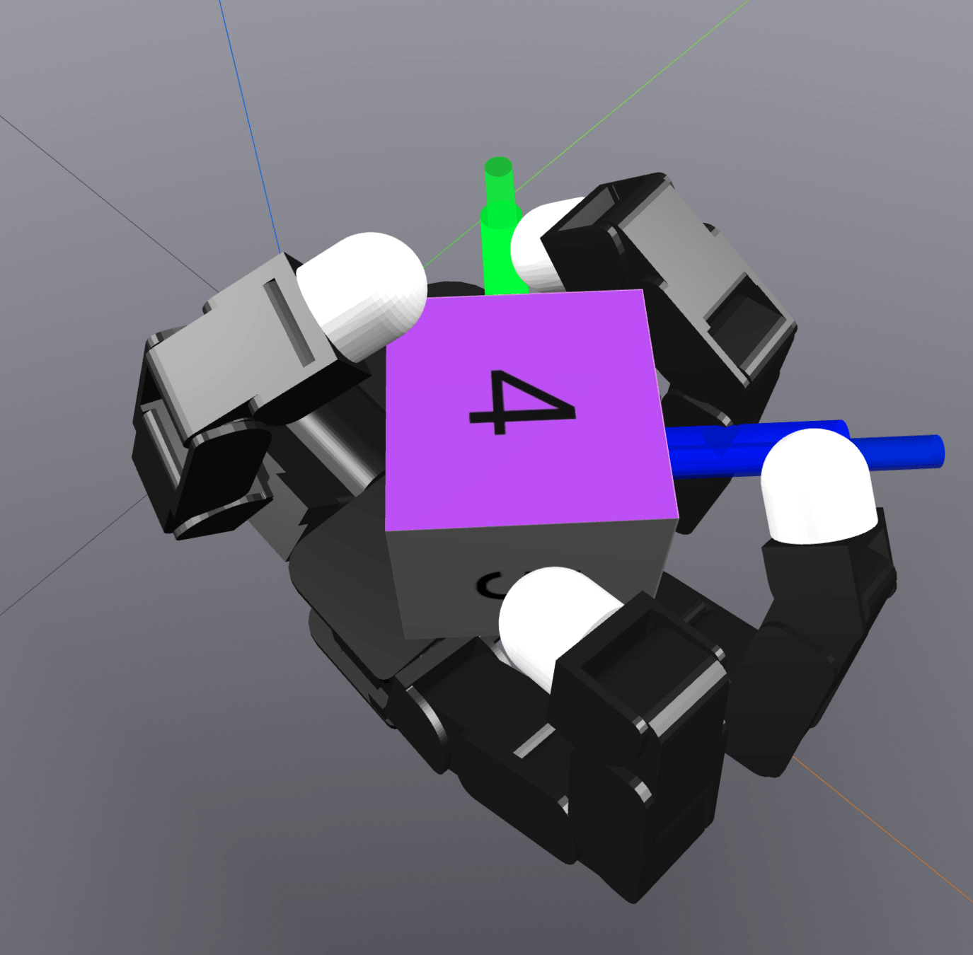
MPC
MPC
Regrasp
(Collision-Free Motion Planning)
Chaining Local Actions
Chaining Local Actions
Conditions for the Framework
- Object is stable during regrasp (Acts like a predicate for the move primitive)
- Local controller is able to correct for small errors while chaining actions together
Roadmap Approach to Manipulation
Offline, build a roadmap of object configuration and keep collection of nominal plans as edges
Roadmap Approach to Manipulation
Roadmap Approach to Manipulation
When getting a new goal that is not in the roadmap, try to connect from nearest node.
[TRO 2023, TRO 2025]
Part 3. Global Planning for Contact-Rich Manipulation
What are fundamental limits of local control?
How can we address difficult exploration problems?
How do we achieve better global planning?


Part 3. Global Planning for Contact-Rich Manipulation
Part 2. Local Planning / Control via Dynamic Smoothing
Part 1. Understanding RL with Randomized Smoothing

Introduction

Preview of Results
Our Method


Contact Scalability
Efficiency
Global Planning

60 hours, 8 NVidia A100 GPUs
5 minutes, 1 Macbook CPU

Thesis Defense (XX)
By Terry Suh
Thesis Defense (XX)
- 633


