Machine Learning!
author : thomaswang
Introduction to Machine Learning
機器學習能幹嘛??
- 解決人類找不出規律的問題
- 語音辨識
- 影像辨識
- 數值預測
- 自駕車
- 金融分析
- 機器人
- 腦波分析
我真的寫得出ML嗎?
- 程式碼-抄 code !
- 資料庫-網路上很多!
- 結論-前人都幫你寫好了!
那我們到底要上什麼???
課程大綱
- 介紹AI、ML
- 類神經元的數學模型
- 類神經網路背後的數學
- 實作機器學習
- 介紹常用的幾種神經網路
學期目標
- 瞭解ML的運作原理
- 看懂程式碼在幹嘛
- 善用網路上的資料庫
- 學習調整ML模型
What is AI ?????
人工智慧(Artificial Intelligence)
人工智慧亦稱智械、機器智慧,指由人製造出來的機器所表現出來的智慧。通常人工智慧是指透過普通電腦程式來呈現人類智慧的技術。(維基百科)
這是人工智慧

這是人工智慧

這也是人工智慧

這還是人工智慧
#include <bits/stdc++.h>
using namespace std;
int main(){
    int a,b;
    cin>>a>>b;
    if(a>b)
        cout<<a<<" is bigger than "<<b<<endl;
    else if(a==b)
        cout<<a<<" is equal to "<<b<<endl;
    else
        cout<<a<<" is smaller than "<<b<<endl;
    return 0;
}
What is AI ???
強人工智慧
弱人工智慧
- 能推理
- 能解決問題
- 具有知覺
- 有自我意識的
- 不真正擁有智慧
- 不會有自主意識
機器學習
- 實現人工智慧的方法之一
- 概率論、統計學、逼近論、凸分析、計算複雜性理論
- 學習:從已知資料分析獲得規律
人工智慧
handcrafted
machine learning
決策樹、線性回歸、類神經網路、邏輯回歸、支援向量機(SVM)、相關向量機(RVM)
訓練資料
有功能的人工智慧
學習 processing...
機器學習
類神經網路-模仿人腦細胞

類神經網路-模仿人腦細胞

神經元
訊號
類神經網路-模仿人腦細胞
類神經網路-模仿人腦細胞
神經元
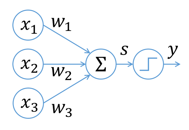
類神經元
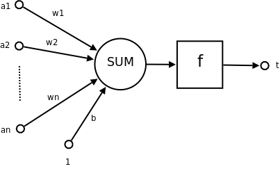
類神經元
-
\(x_1,x_2,x_3\):前面神經元的放電大小
-
\(w_1,w_2,w_3\):前面神經元對這個神經元的影響大小(距離)
-
\(\Sigma x_iw_i\):將前面的影響加總
-
激勵函數:整合前面的影響,向下一個神經元輸出
模仿複雜的細胞???
- 腦細胞真的是這樣運作的嗎?會不會太簡化了?
- 你怎麼確定他做得到?
- 不能模仿得像一點嗎?
- 原來人類就是這樣學習的?
事實上\(\cdots\)
這些算式都是由假設推導出來的
先來瞭解我們的工具吧!!!
之後再慢慢解釋吧\(\cdots\)

學習資源
來玩玩看吧
import numpy as np
import keras
from keras.models import Sequential
from keras.layers import Dense, Dropout, Activation
from keras.optimizers import SGD
import matplotlib.pyplot as plt
# Generate data
d=4
x_train=np.random.random((10000,d))
y_train=[]
x_test=np.random.random((1000,d))
y_test=[]
for i in x_train:
    t=0
    for j in range(d):
        t=t+j*i[j]
    y_train.append(t)
for i in x_test:
    t=0
    for j in range(d):
        t=t+j*(i[j]**j)
    y_test.append(t)

# training
model = Sequential()
model.add(Dense(100, input_dim=d))
model.add(Dense(1))
model.compile(loss='mse',
              optimizer='Adam',
              metrics=['mse'])
model.summary()
history=model.fit(x_train, y_train, epochs=10, batch_size=10, validation_split=0.2)
score = model.evaluate(x_test, y_test, batch_size=64)
print(f"score: {score}")

plt.plot(history.history['loss'])
plt.plot(history.history['val_loss'])
plt.title('Model loss')
plt.ylabel('Loss')
plt.xlabel('Epoch')
plt.legend(['Train', 'Test'], loc='upper right')
plt.show()
來玩玩看吧
# generating training and testing data
import keras
from keras.models import Sequential
from keras.layers import Dense, Dropout, Activation
import numpy as np
import random as rd
import matplotlib.pyplot as plt

d=2
n=1000
test_n=100
x_train=[]
y_train=[]
x_test=[]
y_test=[]
mua=[-2,2]
mub=[2,-2]
sigma=[[5,0],[0,5]]
for i in range(n):
    if rd.randint(0,1)==0:
        x_train.append(np.random.multivariate_normal(mua,sigma))
        y_train.append([1,0])
    else:
        x_train.append(np.random.multivariate_normal(mub,sigma))
        y_train.append([0,1])
for i in range(test_n):
    if rd.randint(0,1)==0:
        x_test.append(np.random.multivariate_normal(mua,sigma))
        y_test.append([1,0])
    else:
        x_test.append(np.random.multivariate_normal(mub,sigma))
        y_test.append([0,1])
x_train=np.array(x_train)
y_train=np.array(y_train)
x_test=np.array(x_test)
y_test=np.array(y_test)

for i in range(n):
    if y_train[i][0]==0:
        plt.scatter(x_train[i][0],x_train[i][1],c="red",marker=".")
    else:
        plt.scatter(x_train[i][0],x_train[i][1],c="blue",marker=".")
plt.show()
# training

import keras
from keras.models import Sequential
from keras.layers import Dense, Dropout, Activation

model = Sequential()
model.add(Dense(100, input_dim=d, activation='sigmoid'))
model.add(Dense(100, input_dim=d, activation='sigmoid'))
model.add(Dense(100, input_dim=d, activation='sigmoid'))
model.add(Dense(100, input_dim=d, activation='sigmoid'))
model.add(Dense(100, input_dim=d, activation='sigmoid'))
model.add(Dense(2,activation='softmax'))
model.compile(loss='categorical_crossentropy',
              optimizer='adam',
              metrics=['accuracy'])
model.summary()
history=model.fit(x_train, y_train, epochs=50, batch_size=128, validation_split=0.2)
score = model.evaluate(x_test, y_test, batch_size=128)
print(f"score: {score}")

# Plot training & validation accuracy values
plt.plot(history.history['acc'])
plt.plot(history.history['val_acc'])
plt.title('Model accuracy')
plt.ylabel('Accuracy')
plt.xlabel('Epoch')
plt.legend(['Train', 'Test'], loc='upper right')
plt.show()

# Plot training & validation loss values
plt.plot(history.history['loss'])
plt.plot(history.history['val_loss'])
plt.title('Model loss')
plt.ylabel('Loss')
plt.xlabel('Epoch')
plt.legend(['Train', 'Test'], loc='upper right')
plt.show()
這堂課大概是\(\cdots\)
- 前面幾堂講ML的數學原理
- 自己寫一兩個ML
- 進入模板+抄code階段!!
數學撐過去就好了!!
brief introduction
to neural network
神經
網路
history of deep learning
- 1958: Perceptron (linear model)
- 1969: Perceptron has limitation
- 1980s: Multi-layer perceptron
- Do not have significant difference from DNN today
- 1986: Backpropagation
- Usually more than 3 hidden layers is not helpful
- 1989: 1 hidden layer is “good enough”, why deep?
- 2006: RBM initialization (breakthrough)
- 2009: GPU
- 2011: Start to be popular in speech recognition
- 2012: win ILSVRC image competition

ImageNet Large Scale Visual Recognition Competition
Universal approximation theorem
通用近似定理
the universal approximation theorem states that a feed-forward network with a single hidden layer containing a finite number of neurons can approximate continuous functions on compact subsets of \(\R^n\), under mild assumptions on the activation function.
- one hidden layer can approximate any function
- why deep ???
- possible , but not feasible!
some tasks
image classification

cat

cat

dog

dog
image classification
INPUT
OUTPUT
predict function
\(f(x)\)

machine learning
1.define
function set
2.find the
best of them
\(a(x)\)
\(b(x)\)
\(h(x)\)
\(z(x)\)
\(l(x)\)
\(o(x)\)
\(y(x)\)
| function | error |
|---|---|
| a(x) | 0.98 |
| b(x) | 40 |
| g(x) | 7122 |
| h(x) | 0.001 |
| y(x) | 90 |
| z(x) | 127 |
function set-neural network
\(x_0\)
\(x_1\)
\(x_2\)
\(x_3\)
\(a_0\)
\(a_1\)
\(a_2\)
\(a_4\)
\(a_5\)
\(c_0\)
\(c_1\)
\(c_2\)
\(c_4\)
\(c_5\)
\(y_1\)
\(y_2\)
\(\cdots\)
so
many
layers
\(\vdots\)
\(\vdots\)
class 1
\(1\)
\(1\)
\(1\)
\(0\)
picture
update parameters due to error
\(0.3\)
\(0.7\)
ans
\(1\)
\(0\)
error
speech recognition
night
animal
baby
smell


speech recognition
night
\begin{bmatrix}
0\\
100\\
6\\
8\\
-100\\
-30\\
\vdots\\
-30\\
10
\end{bmatrix}
Neural
Network
output
input
generate pictures

robot


Artist Robot
How to do that?
painter
teacher

\(1^{st}\) try
terrible !!!

\(3^{rd}\) try
not exactly right
\(2^{nd}\) try
the right shape

\(4^{th}\) try
perfect !!!
Generative adversarial network
GAN 生成對抗網路
-
painter = generative network(生成網絡)
-
teacher = discriminative network(判別網絡)
-
painter generate pictures similar to true pictures
-
teacher distinguishes generated pictures from true pictures
-
painter tries to fool teacher , increase teacher's error rate
-
the opposites become smarter after rounds(iterations)
Game Robot
train an AI to play games
environment
observation
action
reward

score
frame
shoot,move right
A3C reinforcement learning
Asynchronous Advantage Actor-Critic
-
actor = player
-
critic = assessor(評估員)
-
critic gather informations from observation
-
actor take actions due to figures provided by critic
但是\(\cdots\)別想的那麼簡單
-
類神經元怎麼連?
-
怎麼調整參數?
-
怎麼增加正確率?
-
哪來的訓練資料?
如何用數學建立模型!!!
Neural networks aren't
just black boxes
Linear Regression
機器學習的第一步
機器學習種類
- Regression 數值預測
- classification 分類器
- structure learning 輸出為複雜的結構
直接看例子吧!
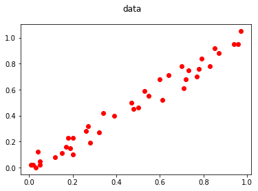
出現新的點該怎麼預測???
\(f(x)\)
\(x\)
\(y\)
what we're looking for
我們該如何找到\(f(x)\)?
- 代公式!!
\(f(x)=wx+b\)
\(w=\frac{\Sigma(x_i-\bar{x})(y_i-\bar{y})}{\Sigma(x_i-\bar{x})^2}\)
\(b=\bar{y}-w\bar{x}\)
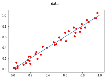
\(y=1.02x-0.009\)
機器學習就這樣\(\cdots\)?
讓我們換個想法\(\cdots\)
一開始隨機初始值 \(w_0,b_i\)
讀入第一次數據
調整參數變成 \(w_1,b_1\)
讀入第二次數據
調整參數變成 \(w_2,b_2\)
\(\vdots\)
讀入第\(n\)次數據
調整參數變成 \(w_n,b_n\)
NO!!!
這是什麼意思?
- 不斷對資料學習、調整
- 回歸線越來越佳
但是他要怎麼學習\(\cdots\)?
機器學習 通常怎麼做?
- 設計函數集合
- 定義誤差函數
- 調整函數
設計函數集合\(f_{\theta_1,\theta_1,\cdots,\theta_k}(x)\)
\(f_{a,b,c}(x)=ax^2+bx+c\)
\(f_{2,15,78}(x)=2x^2+15x+78\)
\(f_{1,2,1}(x)=1x^2+2x+1\)
\(\in\)
\(f_{0,0,0}(x)=0x^2+0x+0\)
\(f_{7,1,22}(x)=7x^2+1x+22\)
\(f_{7,12,2}(x)=7x^2+12x+2\)
\(f_{71,2,2}(x)=71x^2+2x+2\)
\(f_{w,b}(x)=wx+b\)
\(f_{1,2}(x)=1x+2\)
\(f_{2,\pi}(x)=2x+\pi\)
\(\in\)
\(f_{0,0}(x)=0x+0\)
\(f_{71,22}(x)=71x+22\)
\(f_{7,122}(x)=7x+122\)
\(f_{712,2}(x)=712x+2\)
假設線性函數\(f(x)=wx+b\)
但\(\cdots\)你怎麼知道是線性?
定義誤差函數\(L(f_{\theta_1,\theta_2,\cdots,\theta_k})\)
絕對值誤差 \(f(x)\)
\(|f(x)-y|\)
均方誤差 \(f(x)\)
\((f(x)-y)^2\)
cross entropy \(f(\vec{x})=f(x_1,x_2,\cdots,x_n)\)
\(-\sum f(x_i)\log y_i\)
\(L(f_{w,b})=\frac{1}{n}\sum(f_{w,b}(x_i)-y_i)^2\)
調整函數
\[ f_1(x)\rightarrow f_2 (x)\rightarrow\cdots\rightarrow f_n(x)\]
假如我們窮舉所有\(w\)和\(b\)?
- 消耗太多時間
- \(w,b\)沒有範圍限制!!
\(\Longrightarrow\)不可能窮舉!!
發揮一些想像力\(\cdots\)
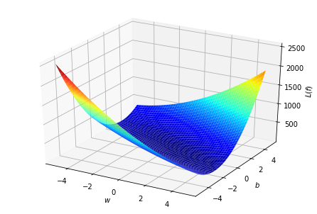
取\(\log\)看得更清楚
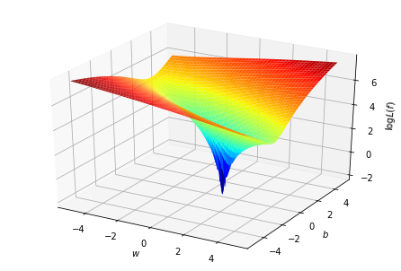
最佳函數
在空間中找到最低點
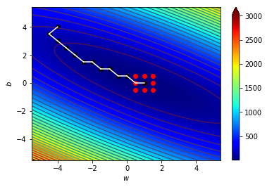
\(\Rightarrow\)不斷向低的方向走
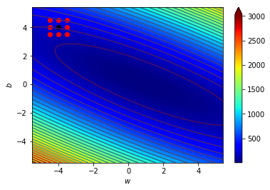
初始\((w,b)\)
\((w,b)\)代表\(f_{w,b}(x)\)
尋找\((w\pm\Delta,b),(w,b\pm\Delta),(w\pm\Delta,b\pm\Delta)\)哪一個最好
移動單位\(\Delta\)越小,結果越精準
若\((w,b)\)已是四周最小的,則\(f_{w,b}(x)為最好的函數\)
否則\((w,b)\)更新為四周最好的那組
以相同方法繼續更新\((w,b)\)
什麼東西???好抽象喔
看圖更清楚
\((w_0,b_0)=(-4,4)\),\(\Delta=0.5\)
\((w_1,b_1)=(-4.5,3.5)\),\(\Delta=0.5\)

\((w_2,b_2)=(-4,3)\),\(\Delta=0.5\)

\((w_3,b_3)=(-3.5,2.5)\),\(\Delta=0.5\)

\((w_4,b_4)=(-3,2)\),\(\Delta=0.5\)

\((w_5,b_5)=(-2.5,1.5)\),\(\Delta=0.5\)

\((w_6,b_6)=(-2,1.5)\),\(\Delta=0.5\)

\((w_7,b_7)=(-1.5,1)\),\(\Delta=0.5\)
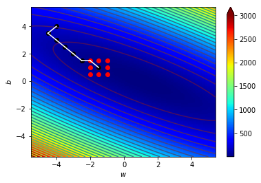
\((w_8,b_8)=(-1,1)\),\(\Delta=0.5\)

\((w_9,b_9)=(-0.5,0.5)\),\(\Delta=0.5\)

\((w_{10},b_{10})=(0,0.5)\),\(\Delta=0.5\)
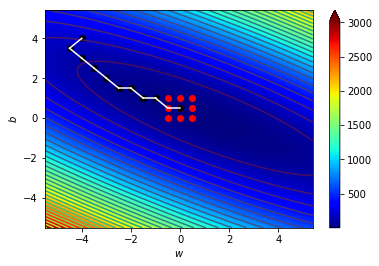
\((w_{11},b_{11})=(0.5,0)\),\(\Delta=0.5\)

\((w_{12},b_{12})=(1,0)\),\(\Delta=0.5\)
當\(\Delta\)更小時
\((w_{final},b_{final})=(1.020,-0.009)\),\(\Delta=0.001\)

\(y=1.02x-0.009\)
一模一樣!!!
import matplotlib.colors as colors
import matplotlib.cm as cm
from matplotlib import animation, rc
from IPython.display import HTML
from mpl_toolkits.mplot3d import Axes3D
import matplotlib.pyplot as plt
import numpy as np
import pandas as pd

# getting training data from github
url = 'https://thomasinfor.github.io/train-data/linear_regression1.csv'
data = pd.read_csv(url)
x=np.array(data['x'])
y=np.array(data['y'])
n=len(x)

# define loss function and best-point function
def loss(w,b):
    total=0
    for i in range(n):
        total=total+(w*x[i]+b-y[i])**2
    return total/n

delta=0.001
def p(w,b):
    pnt=(w,b)
    for dw in range (-1,2):
        for db in range (-1,2):
            if loss(pnt[0],pnt[1])>loss(w+dw*delta,b+db*delta):
                pnt=(w+dw*delta,b+db*delta)
        trace.append(pnt)
    return pnt
point=(-4,4)
trace=[[point[0]],[point[1]],[loss(point[0],point[1])]]

# train!!!
while True:
    # get the best point around
    temp=p(point[0],point[1])
    # break the loop if the current
    # point is already the best
    if(temp==point):
        break;
    # step to the best point
    point=temp
    # adding the trace for plotting
    trace[0].append(point[0])
    trace[1].append(point[1])
    trace[2].append(loss(point[0],point[1]))

print(f"result: w = {point[0]} , b = {point[1]}")

# plotting result
# you can just ignore this part when
# you're reading as an beginner
fig, ax = plt.subplots(1,2)
fig.patch.set_alpha(0)
fig.set_size_inches(fig.get_figwidth()*2,fig.get_figheight())
plt.close()
ax[0].set_xlim(-0.1*len(trace[0]),len(trace[0])*1.1)
ax[0].set_ylim(-0.1*max(trace[2]),max(trace[2])*1.1)
ax[1].set_xlabel('$iteration$')
ax[1].set_ylabel('$loss$')
X = np.linspace(-6, 6, 100)
Y = np.linspace(-6, 6, 100)
X, Y = np.meshgrid(X, Y)
Z = Y * 0
for i in range(n):
    Z = Z + (X*x[i]+Y-y[i])**2
pcm = ax[1].pcolor(X, Y, Z, norm=colors.Normalize(vmin=Z.min(), vmax=Z.max()), cmap=cm.jet)
ax[1].contour(X,Y,Z,30)
fig.colorbar(pcm, ax=ax, extend='max')
ax[0].set_xlabel('$iteration$')
ax[0].set_ylabel('$loss$')
ax[1].set_xlabel('$w$')
ax[1].set_ylabel('$b$')
x0, y0 = [], []
x1, y1 = [], []
line0, = ax[0].plot([],[],c='black')
line1, = ax[1].plot([],[],c='white')
def animate(i):
    x0.append(i)
    y0.append(trace[2][int(i)])
    x1.append(trace[0][int(i)])
    y1.append(trace[1][int(i)])
    line0.set_data(x0,y0)
    line1.set_data(x1,y1)
    return (line0,line1)
anim = animation.FuncAnimation(fig, animate, frames=np.linspace(0,len(trace[0])-1,100), interval=30, blit=True)
rc('animation', html='jshtml')
anim
想必這就是機器學習了吧!
NO!!!
還可以更優化呢!
-
坡度越陡,移動越遠
-
向任意方向延伸
\(\Longrightarrow\) 微分!!!
下集待續
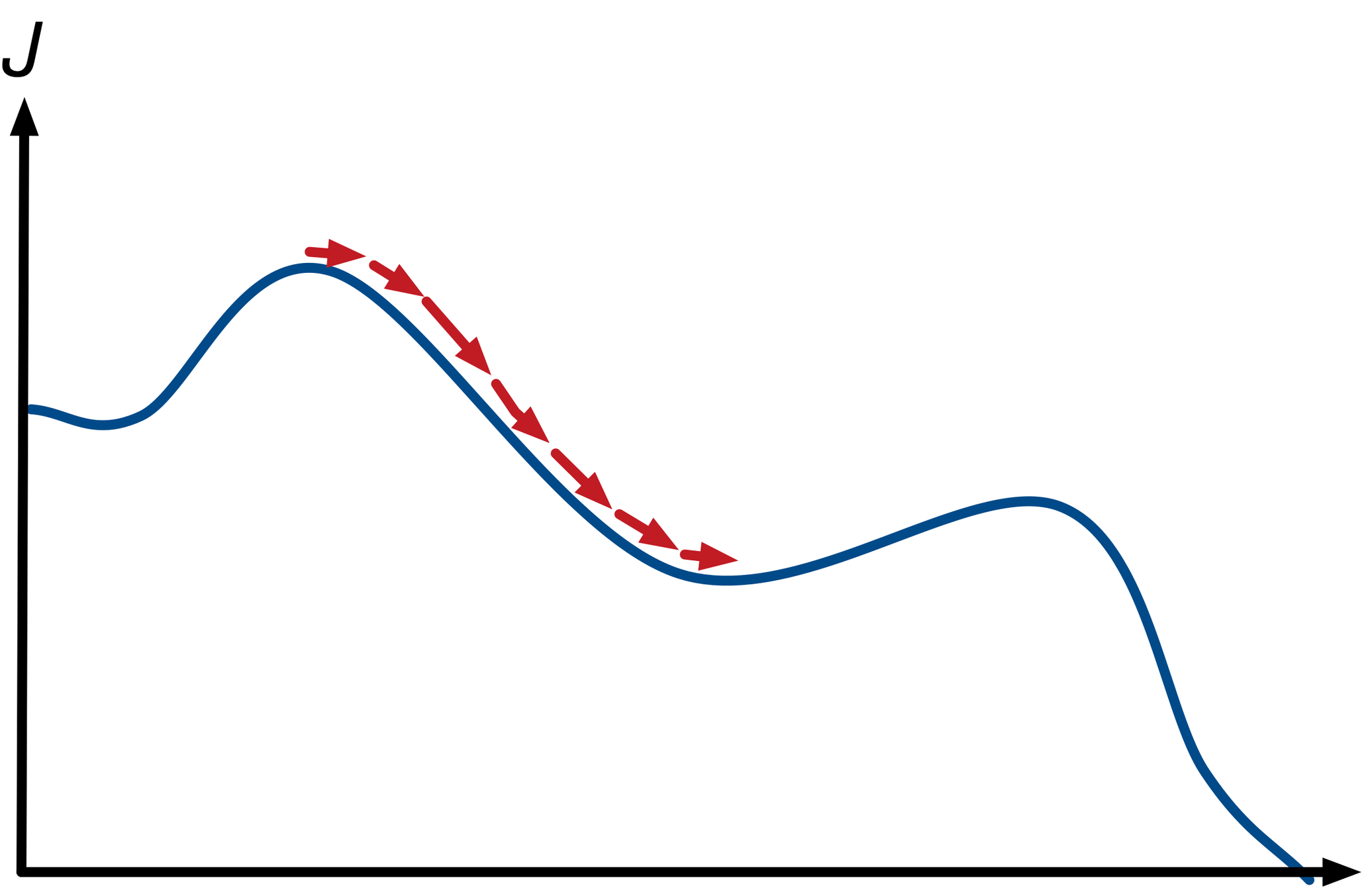
Gradient Descent
梯度下降法
核心想法
-
傾斜程度越大,移動越遠
-
向任意方向延伸(非網格狀)
微分!
往坡度低的方向走
坡度 \(=\frac{\Delta y}{\Delta x}=\) 微分值
\(\Delta x=3\)
\(\Delta x=-1\)
\(\Delta y=2\)
\(\Delta y=3\)
坡度\(=\frac{2}{3}\)
坡度\(=\frac{3}{-1}\)
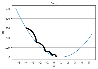
上次我們這樣做
\(w\)
\(loss\)
finished !!!
\(b\)
核心想法
\(w_0,b\)
\(w_1,b\)
\(w_2,b\)
\(w_3,b\)
\(w_4,b\)
核心想法
\(w_{n+1}=w_n+\Delta w\)
\(\Delta w\propto \frac{\partial L(f)}{\partial w}\)
\(\Delta w=-\eta \frac{\partial L(f)}{\partial w}\)
\(\Delta w\):參數更新量
\(\frac{\partial L(f)}{\partial w}\):偏微分值
核心想法
\(b_{n+1}=b_n+\Delta b\)
\(\Delta b\propto \frac{\partial L(f)}{\partial b}\)
\(\Delta b=-\eta \frac{\partial L(f)}{\partial b}\)
\(\Delta b\):參數更新量
\(\frac{\partial L(f)}{\partial b}\):偏微分值
\(\eta\):學習速率(某常數)
\(L(f)=\frac{1}{n}\sum(f(x_i)-y_i)^2=\frac{1}{n}\sum(wx_i+b-y_i)^2\)
\(\frac{\partial L(f)}{\partial w}=\frac{\partial L(f)}{\partial f}\frac{\partial f}{\partial w}\)
\(=\frac{2}{n}\sum(f(x_i)-y_i)(x_i)\)
\(\frac{\partial L(f)}{\partial b}=\frac{\partial L(f)}{\partial f}\frac{\partial f}{\partial b}\)
\(=\frac{2}{n}\sum(f(x_i)-y_i)\)
import matplotlib.colors as colors
import matplotlib.cm as cm
from matplotlib import animation, rc
from IPython.display import HTML
from mpl_toolkits.mplot3d import Axes3D
import matplotlib.pyplot as plt
import numpy as np
import pandas as pd
import time
# getting training data from github
url = 'https://thomasinfor.github.io/train-data/linear_regression1.csv'
data = pd.read_csv(url)
x=np.array(data['x'])
y=np.array(data['y'])
n=len(x)
# define loss function
def loss(w,b):
total=0
for i in range(n):
total+=(w*x[i]+b-y[i])**2
return total/n
# define differatial
def dldw(w,b):
total=0
for i in range(n):
total+=(w*x[i]+b-y[i])*x[i]
return total/n
# define differatial
def dldb(w,b):
total=0
for i in range(n):
total+=(w*x[i]+b-y[i])
return total/n
# initialize
w=-4
b=4
trace=[[w],[b],[loss(w,b)]]
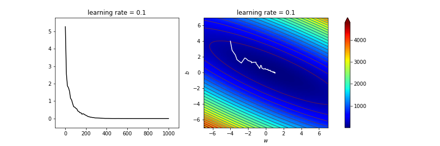
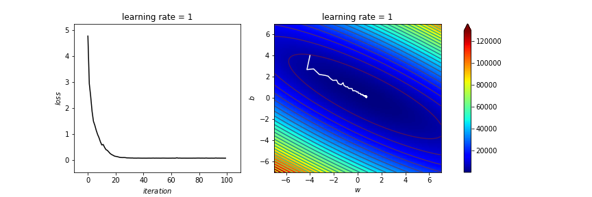
learning_rate=1
# 1.65 1.6 1.5 1 0.1 0.01
# train!!!
iters=100
start=time.time()
for iteration in range(iters):
last=(w,b)
w-=learning_rate*dldw(last[0],last[1])
b-=learning_rate*dldb(last[0],last[1])
# if ((last[0]-w)**2+(last[1]-b)**2)<0.00000001:
# break;
trace[0].append(w)
trace[1].append(b)
trace[2].append(loss(w,b))
print("finished")
end=time.time()
print(f"time: {end-start} sec.")
print(f"result: w = {w} , b = {b}")
# plotting result
# you can just ignore this part when
# you're reading as an beginner
fig, ax = plt.subplots(1,2)
fig.patch.set_alpha(0)
fig.set_size_inches(fig.get_figwidth()*2,fig.get_figheight())
plt.close()
ax[0].set_xlim(-iters*0.1,iters*1.1)
ax[0].set_ylim(-0.1*max(trace[2]),max(trace[2])*1.1)
ax[1].set_xlabel('$iteration$')
ax[1].set_ylabel('$loss$')
X = np.linspace(-7, 7, 100)
Y = np.linspace(-7, 7, 100)
X, Y = np.meshgrid(X, Y)
Z = Y * 0
for i in range(n):
Z = Z + (X*x[i]+Y-y[i])**2
pcm = ax[1].pcolor(X, Y, Z, norm=colors.Normalize(vmin=Z.min(), vmax=Z.max()), cmap=cm.jet)
ax[1].contour(X,Y,Z,30)
fig.colorbar(pcm, ax=ax, extend='max')
ax[0].set_xlabel('$iteration$')
ax[0].set_ylabel('$loss$')
ax[1].set_xlabel('$w$')
ax[1].set_ylabel('$b$')
x0, y0 = [], []
x1, y1 = [], []
line0, = ax[0].plot([],[],c='black')
line1, = ax[1].plot([],[],c='white')
def animate(i):
x0.append(i)
y0.append(trace[2][int(i)])
x1.append(trace[0][int(i)])
y1.append(trace[1][int(i)])
line0.set_data(x0,y0)
line1.set_data(x1,y1)
return (line0,line1)
anim = animation.FuncAnimation(fig, animate, frames=iters, interval=30, blit=True)
rc('animation', html='jshtml')
anim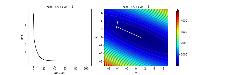
寫了那麼多 不是代公式就好了嗎?
\(f(x)=wx+b\)
\(w=\frac{\sum(x_i-\bar{x})(y_i-\bar{y})}{\sum(x_i-\bar{x})^2}\)
\(b=\bar{y}-w\bar{x}\)
梯度下降的優點
- 多維空間也適用!
- 可微分函數都適用!
- 非網格狀(無最小單位)
\(\Longrightarrow\)可處理更複雜的函數
多維空間\(f(\vec{x})=f(x_1,x_2,\cdots,x_d)\)
\(f(\vec{x})=f(x_1,x_2,\cdots,x_d)\)
\(=w_1x_1+w_2x_2+\cdots+w_dx_d+b\)
\(=\sum w_ix_i+b=\vec{w}\cdot\vec{x}+b\)
線性回歸
\(L(f)=\frac{1}{n}\Sigma(f(\vec{x_i})-y_i)^2=\frac{1}{n}\Sigma(\vec{w}\cdot\vec{x_i}+b-y_i)^2\)
\(\frac{\partial L(f)}{\partial w_i}=\frac{\partial L(f)}{\partial f}\frac{\partial f}{\partial w_i}\)
\(=\frac{2}{n}\Sigma(f(\vec{x_j})-y_j)(x_{j,i})\)
\(\frac{\partial L(f)}{\partial b}=\frac{\partial L(f)}{\partial f}\frac{\partial f}{\partial b}\)
\(=\frac{2}{n}\Sigma(f(\vec{x_j})-y_j)\)
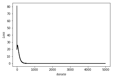
\(9\)維資料線性回歸
import matplotlib.pyplot as plt
import matplotlib.colors as colors
import matplotlib.cm as cm
import numpy as np

d=10
n=40
x=[[0.99, 0.15, 0.15, 0.31, 0.78, 0.78, 0.87, 0.3, 0.46], [0.91, 0.05, 0.58, 0.99, 0.41, 0.49, 0.98, 0.29, 0.3], [0.61, 0.52, 0.01, 0.85, 0.74, 0.64, 0.08, 0.7, 0.93], [0.1, 0.14, 0.06, 0.1, 0.61, 0.97, 0.39, 0.72, 0.7], [0.51, 0.67, 0.19, 0.65, 0.2, 0.71, 0.2, 0.08, 0.41], [0.2, 0.4, 0.79, 0.45, 0.83, 0.95, 0.56, 0.89, 0.66], [0.12, 0.84, 0.59, 0.96, 0.1, 0.48, 0.17, 0.82, 0.38], [0.95, 0.3, 0.44, 0.02, 0.34, 0.12, 0.38, 0.87, 0.9], [0.3, 0.78, 0.19, 0.71, 0.13, 0.63, 0.49, 0.49, 0.67], [0.07, 0.82, 0.04, 0.55, 0.11, 0.68, 0.32, 0.11, 0.45], [0.85, 0.52, 0.3, 0.39, 0.2, 0.88, 0.88, 0.26, 0.46], [0.46, 0.97, 0.49, 0.24, 0.76, 0.24, 0.05, 0.25, 0.82], [0.68, 0.04, 0.32, 0.71, 0.63, 0.33, 0.72, 0.47, 0.62], [0.96, 0.4, 0.64, 0.54, 0.3, 0.54, 0.8, 0.13, 0.61], [0.33, 0.62, 0.01, 0.15, 0.98, 0.8, 0.64, 0.78, 0.82], [0.05, 0.51, 0.94, 0.26, 0.46, 0.77, 0.22, 0.86, 0.21], [0.25, 0.43, 0.95, 0.1, 0.33, 0.86, 0.26, 0.04, 0.94], [0.37, 0.62, 0.16, 0.53, 0.55, 0.2, 0.04, 0.0, 0.8], [0.59, 0.59, 0.0, 0.32, 0.64, 0.28, 0.04, 0.0, 0.83], [0.17, 0.53, 0.62, 0.78, 0.7, 0.28, 0.2, 0.68, 0.45], [0.08, 0.38, 0.44, 0.22, 0.83, 0.85, 0.55, 0.87, 0.26], [0.24, 0.7, 0.57, 0.64, 0.5, 0.73, 0.29, 0.0, 0.21], [0.22, 0.25, 0.4, 0.59, 0.3, 0.41, 0.51, 0.54, 0.52], [0.18, 1.01, 0.07, 0.75, 0.14, 0.73, 0.84, 0.23, 0.69], [0.25, 0.39, 0.15, 0.92, 0.03, 0.84, 0.6, 0.3, 0.48], [0.89, 0.33, 0.8, 0.2, 0.11, 0.88, 0.91, 0.63, 0.53], [0.76, 0.14, 0.48, 0.53, 0.1, 0.7, 0.34, 0.39, 0.11], [0.68, 0.03, 0.81, 0.88, 0.15, 0.19, 0.58, 0.41, 0.36], [0.55, 0.17, 0.04, 0.28, 0.18, 0.58, 0.7, 0.6, 0.03], [0.65, 0.03, 0.57, 0.28, 0.42, 0.46, 0.27, 0.33, 0.37], [0.63, 0.47, 0.29, 0.27, 0.93, 0.44, 0.28, 0.49, 0.91], [0.87, 0.23, 0.95, 0.87, 0.06, 0.31, 0.67, 0.81, 0.53], [0.12, 0.55, 0.59, 0.87, 0.83, 0.76, 0.79, 0.86, 0.81], [0.13, 0.97, 0.16, 0.23, 0.46, 0.13, 0.43, 0.69, 0.66], [0.07, 0.62, 0.87, 0.78, 0.93, 0.54, 0.89, 0.36, 0.79], [0.34, 0.6, 0.86, 0.33, 0.56, 0.28, 0.94, 0.51, 0.72], [0.31, 0.68, 0.94, 0.53, 0.07, 0.38, 0.11, 0.85, 0.15], [0.37, 0.2, 0.41, 0.5, 0.56, 0.78, 0.39, 0.99, 0.27], [0.21, 0.12, 0.38, 0.64, 0.81, 0.94, 0.25, 0.62, 0.23], [0.43, 0.78, 0.81, 0.32, 0.18, 0.57, 0.48, 0.62, 0.64]]
y=[28.4, 27.58, 31.07, 29.83, 21.39, 35.269999999999996, 26.499999999999996, 27.77, 27.689999999999998, 21.680000000000003, 27.270000000000003, 24.52, 28.549999999999997, 26.79, 33.87, 26.88, 26.61, 21.37, 21.39, 26.87, 29.96, 21.83, 26.07, 28.779999999999998, 26.31, 30.479999999999997, 21.240000000000002, 24.069999999999997, 22.349999999999998, 21.88, 29.17, 29.46, 37.7, 26.160000000000004, 34.3, 30.92, 23.139999999999997, 29.09, 27.419999999999998, 28.27]
def ip(a,b):
  t=0
  for i in range(len(a)):
    t=t+a[i]*b[i]
  return t
def l(w,b):
  t=0
  for i in range(n):
    t=t+(ip(w,x[i])+b-y[i])**2
  return t/n
def dldw(w,b,j):
  k=0
  for i in range(n):
    k=k+(ip(w,x[i])+b-y[i])*x[i][j]
  return k/n;
def dldb(w,b):
  k=0
  for i in range(n):
    k=k+(ip(w,x[i])+b-y[i])
  return k/n;
w=[]
b=0
for i in range(d-1):
  w.append(0)
t=[[w,b]]
fig, ax = plt.subplots()
lr=0.5
for cnt in range(5000):
  last=(w,b)
  for i in range(d-1):
    w[i]=w[i]-lr*dldw(w,b,i)
  b=b-lr*dldb(w,b)
  t.append([w,b])
for i in range(len(t)-1):
  plt.plot([i,i+1],[l(t[i][0],t[i][1]),l(t[i+1][0],t[i+1][1])],c="black")
ax.set_xlabel('$iterate$')
ax.set_ylabel('$Loss$')
plt.show()
print(w)
print(b)
print(l(w,b))
多項式回歸
\(f(x)=a_0+a_1x+a_2x^2+\cdots+a_nx^n\)
\(=\sum a_ix^i\)
\(\)
非線性函數回歸
\(L(f)=\frac{1}{n}\sum(f(x_i)-y_i)^2=\frac{1}{n}\sum(\sum a_ix^i-y_i)^2\)
\(\frac{\partial L(f)}{\partial a_i}=\frac{\partial L(f)}{\partial f}\frac{\partial f}{\partial a_i}\)
\(=\frac{2}{n}\sum(f(x_j)-y_j)(x^i)\)
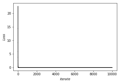
多項式回歸
import matplotlib.pyplot as plt
import matplotlib.colors as colors
import matplotlib.cm as cm
import numpy as np

d=5
n=100
x=[0.76, 0.96, 0.94, 0.02, 0.25, 0.88, 0.92, 0.99, 0.38, 0.67, 0.48, 0.69, 0.57, 0.98, 0.1, 0.41, 0.47, 0.71, 0.37, 0.58, 1.0, 0.64, 0.15, 0.91, 0.03, 0.96, 0.42, 0.57, 0.93, 0.14, 0.29, 0.11, 0.86, 0.62, 0.98, 0.46, 0.71, 0.65, 0.15, 0.76, 0.27, 0.88, 0.96, 0.07, 0.63, 0.04, 0.31, 0.87, 0.02, 0.91, 0.4, 0.48, 0.27, 0.18, 0.16, 0.27, 0.18, 0.28, 0.98, 0.4, 0.15, 0.71, 0.83, 0.05, 0.98, 0.89, 0.37, 0.25, 0.66, 0.85, 0.68, 0.53, 0.46, 0.19, 0.13, 0.28, 0.16, 0.55, 0.94, 0.63, 0.52, 0.55, 0.83, 0.28, 0.98, 0.62, 1.01, 0.97, 0.43, 0.7, 0.96, 0.31, 0.47, 1.01, 0.61, 0.84, 0.04, 0.13, 0.41, 0.6]
y=[]
for i in range(n):
  t=0
  for j in range(d):
    t=t+j*(x[i]**j)
  y.append(t)
def l(aa):
  t=0
  for i in range(n):
    k=0
    for j in range(d):
      k=k+aa[j]*(x[i]**j)
    t=t+((k-y[i])**2)/n
  return t
def dlda(aa,j):
  t=0
  for i in range(n):
    k=0
    for m in range(d):
      k=k+aa[m]*(x[i]**m)
    t=t+(k-y[i])*(x[i]**j)/n
  return t
a=[]
for i in range(d):
  a.append(0)
t=[list(a)]
fig, ax = plt.subplots()
lr=1
for cnt in range(10000):
  last=list(a)
  for i in range(d):
    a[i]=a[i]-lr*dlda(last,i)
  t.append(list(a))
  plt.plot([cnt,cnt+1],[l(last),l(a)],c="black")
ax.set_xlabel('$iterate$')
ax.set_ylabel('$Loss$')
plt.show()
print(a)
print(l(a))
你是否會覺得學習太慢呢\(\cdots\)?
總共更新\(a\)次、\(n\)組學習資料、\(d\)個參數:
複雜度\(O(a\cdot n\cdot d)\)
剛剛多項式回歸:\(O(10000\times 100\times 10)\Rightarrow 1 min\)
當參數越來越大量\(\cdots\)我們又要優化了
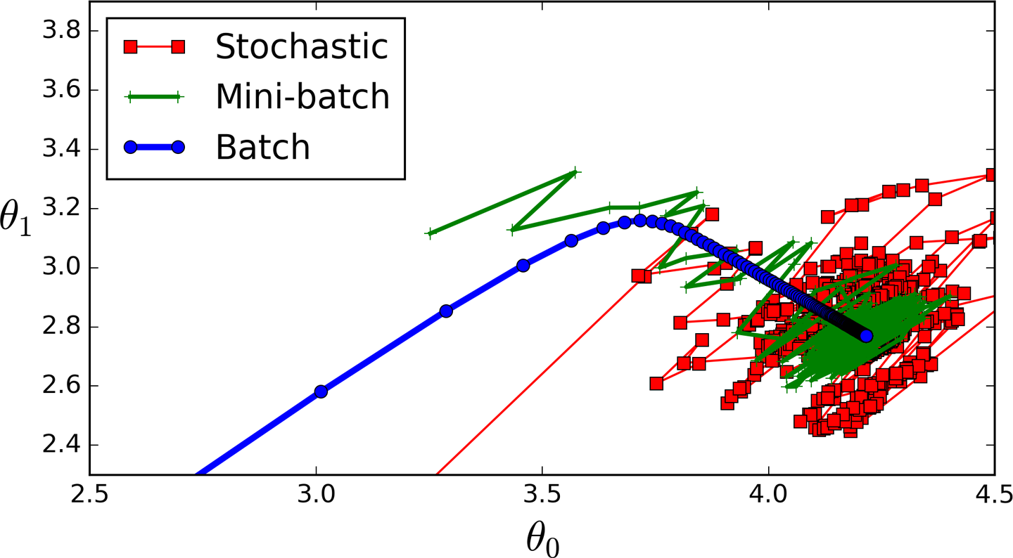
stochastic gradient descent
\(L(f)=\frac{1}{n}\sum(f(x_i)-y_i)^2\)
\(=\Sigma P_i(f(x_i)-y_i)^2 (P_i=\frac{1}{n})\)
\(=E(x)\)
什麼意思???
stochastic gradient descent
每次更新要算一次誤差 \(=\) 跑一次學習資料
浪費時間!
假如我們算誤差時隨機取一組資料來算
期望值\(E(X)=\Sigma P_iX_i\)
\(=\Sigma (\frac{1}{n})(f(x_i)-y_i)^2\)
和誤差公式一模一樣!!
\(\Rightarrow\)用隨機取樣代替全部算一次
import matplotlib.colors as colors
import matplotlib.cm as cm
from matplotlib import animation, rc
from IPython.display import HTML
from mpl_toolkits.mplot3d import Axes3D
import matplotlib.pyplot as plt
import numpy as np
import pandas as pd
import random as rd
import time
# getting training data from github
url = 'https://thomasinfor.github.io/train-data/linear_regression2.csv'
data = pd.read_csv(url)
x=np.array(data['x'])/100
y=np.array(data['y'])/100
n=len(x)
# define loss function
def loss(w,b):
total=0
for i in range(n):
total+=(w*x[i]+b-y[i])**2
return total/n
# define differatial
def dldw(w,b):
i=rd.randint(0,n-1)
return (w*x[i]+b-y[i])*x[i]
# define differatial
def dldb(w,b):
i=rd.randint(0,n-1)
return (w*x[i]+b-y[i])
# initialize
w=-4
b=4
trace=[[w],[b],[]]
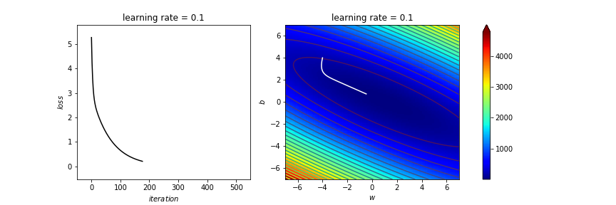
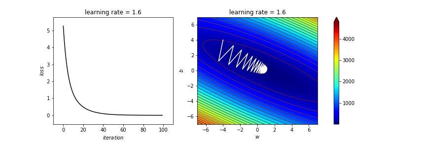
learning_rate=1.4
iters=100
# train!!!
start=time.time()
for iteration in range(iters):
last=(w,b)
w-=learning_rate*dldw(last[0],last[1])
b-=learning_rate*dldb(last[0],last[1])
# if ((last[0]-w)**2+(last[1]-b)**2)<0.00000001:
# break;
trace[0].append(w)
trace[1].append(b)
print("finished")
end=time.time()
print(f"time: {end-start} sec.")
print(f"result: w = {w} , b = {b}")
for i in range(len(trace[0])):
trace[2].append(loss(trace[0][i],trace[1][i]))
# plotting result
# you can just ignore this part when
# you're reading as an beginner
fig, ax = plt.subplots(1,2)
plt.close()
fig.patch.set_alpha(0)
fig.set_size_inches(fig.get_figwidth()*2,fig.get_figheight())
ax[0].set_title('learning rate = '+str(learning_rate))
ax[0].set_xlim(-iters*0.1,iters*1.1)
ax[0].set_ylim(-0.1*max(trace[2]),max(trace[2])*1.1)
ax[1].set_title('learning rate = '+str(learning_rate))
ax[1].set_xlabel('$iteration$')
ax[1].set_ylabel('$loss$')
X = np.linspace(-7, 7, 100)
Y = np.linspace(-7, 7, 100)
X, Y = np.meshgrid(X, Y)
Z = Y * 0
for i in range(n):
Z = Z + (X*x[i]+Y-y[i])**2
pcm = ax[1].pcolor(X, Y, Z, norm=colors.Normalize(vmin=Z.min(), vmax=Z.max()), cmap=cm.jet)
ax[1].contour(X,Y,Z,30)
fig.colorbar(pcm, ax=ax, extend='max')
ax[0].set_xlabel('$iteration$')
ax[0].set_ylabel('$loss$')
ax[1].set_xlabel('$w$')
ax[1].set_ylabel('$b$')
x0, y0 = [], []
x1, y1 = [], []
line0, = ax[0].plot([],[],c='black')
line1, = ax[1].plot([],[],c='white')
def animate(i):
x0.append(i)
y0.append(trace[2][int(i)])
x1.append(trace[0][int(i)])
y1.append(trace[1][int(i)])
line0.set_data(x0,y0)
line1.set_data(x1,y1)
return (line0,line1)
rc('animation', html='jshtml',)
anim = animation.FuncAnimation(fig, animate, frames=np.linspace(0,iters-1,100), interval=30, blit=True)
anim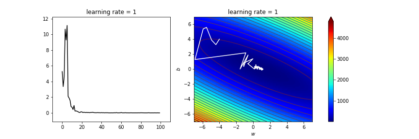
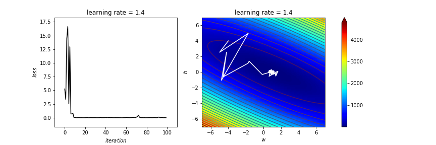
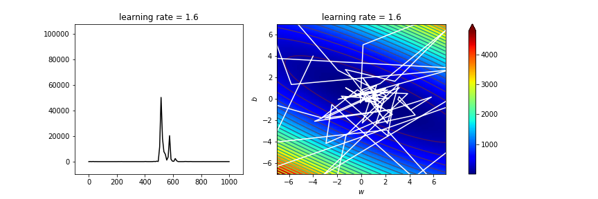
太亂了吧
stochastic gradient descent
mini-batch SGD
雖然期望值與誤差函數相同,但變異太大!
batch size:取幾組資料近似\(L(x)\)
mini-batch:每次更新需要的小資料
利用小資料平均,更接近實際誤差
在誤差和時間中抉擇
import matplotlib.colors as colors
import matplotlib.cm as cm
from matplotlib import animation, rc
from IPython.display import HTML
from mpl_toolkits.mplot3d import Axes3D
import matplotlib.pyplot as plt
import numpy as np
import pandas as pd
import random as rd
import time

batch_size=50

# getting training data from github
url = 'https://thomasinfor.github.io/train-data/linear_regression2.csv'
data = pd.read_csv(url)
x=np.array(data['x'])/100
y=np.array(data['y'])/100
n=len(x)
print(n,'datas')

# define loss function
def loss(w,b):
    total=0
    for i in range(n):
        total+=(w*x[i]+b-y[i])**2
    return total/n
# define differatial
def dldw(w,b):
    total=0
    for cnt in range(batch_size):
        i=rd.randint(0,n-1)
        total+=(w*x[i]+b-y[i])*x[i]
    return total/batch_size
# define differatial
def dldb(w,b):
    total=0
    for cnt in range(batch_size):
        i=rd.randint(0,n-1)
        total+=(w*x[i]+b-y[i])
    return total/batch_size

# initialize
w=-4
b=4
trace=[[w],[b],[]]
learning_rate=1
iters=100

# train!!!
start=time.time()
for iteration in range(iters):
    last=(w,b)
    w-=learning_rate*dldw(last[0],last[1])
    b-=learning_rate*dldb(last[0],last[1])
    # if ((last[0]-w)**2+(last[1]-b)**2)<0.00000001:
    #     break;
    trace[0].append(w)
    trace[1].append(b)
print("finished")
end=time.time()
print(f"time: {end-start} sec.")
print(f"result: w = {w} , b = {b}")

for i in range(len(trace[0])):
    trace[2].append(loss(trace[0][i],trace[1][i]))

# plotting result
# you can just ignore this part when
# you're reading as an beginner
fig, ax = plt.subplots(1,2)
plt.close()
fig.patch.set_alpha(0)
fig.set_size_inches(fig.get_figwidth()*2,fig.get_figheight())
ax[0].set_title('learning rate = '+str(learning_rate))
ax[0].set_xlim(-iters*0.1,iters*1.1)
ax[0].set_ylim(-0.1*max(trace[2]),max(trace[2])*1.1)
ax[1].set_title('learning rate = '+str(learning_rate))
ax[1].set_xlabel('$iteration$')
ax[1].set_ylabel('$loss$')
X = np.linspace(-7, 7, 100)
Y = np.linspace(-7, 7, 100)
X, Y = np.meshgrid(X, Y)
Z = Y * 0
for i in range(n):
    Z = Z + (X*x[i]+Y-y[i])**2
pcm = ax[1].pcolor(X, Y, Z, norm=colors.Normalize(vmin=Z.min(), vmax=Z.max()), cmap=cm.jet)
ax[1].contour(X,Y,Z,30)
fig.colorbar(pcm, ax=ax, extend='max')
ax[0].set_xlabel('$iteration$')
ax[0].set_ylabel('$loss$')
ax[1].set_xlabel('$w$')
ax[1].set_ylabel('$b$')
x0, y0 = [], []
x1, y1 = [], []
line0, = ax[0].plot([],[],c='black')
line1, = ax[1].plot([],[],c='white')
def animate(i):
    x0.append(i)
    y0.append(trace[2][int(i)])
    x1.append(trace[0][int(i)])
    y1.append(trace[1][int(i)])
    line0.set_data(x0,y0)
    line1.set_data(x1,y1)
    return (line0,line1)
rc('animation', html='jshtml',)
anim = animation.FuncAnimation(fig, animate, frames=np.linspace(0,iters-1,100), interval=30, blit=True)
anim
linear regression
batch size \(=50\)
時間差別
| linear | 10D | polynomial | |
|---|---|---|---|
| before | 30s | 48s | 222s |
| after | 11s | 10s | 17s |
| dataset | 1000 | 500 | 1000 |
| batchsize | 50 | 50 | 50 |
節省大量時間!!
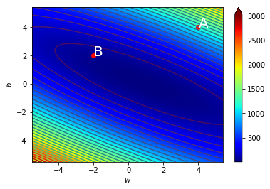
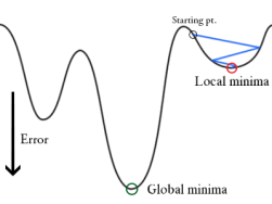
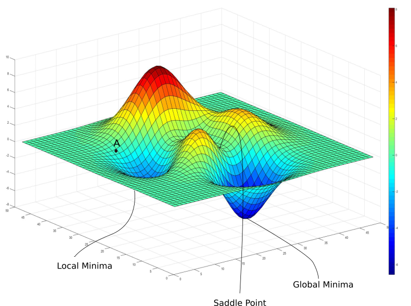
Some Problems
global minima v.s. local minima
最小值
極小值
global minima v.s. local minima
global minima v.s. local minima
global minima v.s. local minima
global minima v.s. local minima
global minima v.s. local minima
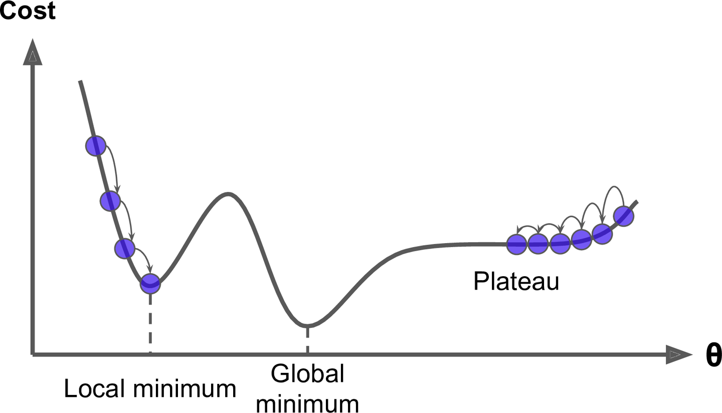
- 梯度下降法未必能停在最低點
- 不同初始位置會停在不同極小
事實上\(\cdots\)
不可能確定最小值在哪!!!
solution
以後再說
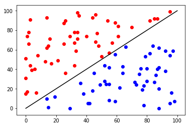
Logistic Regression
邏輯回歸
last time\(\cdots\)
坡度緩,走慢一點
坡度陡,走快一點
last time\(\cdots\)
移動距離正比於坡度
偏微分算坡度!
\Delta\theta\text{(移動距離)}=-\eta\text{(學習速率)}\times\frac{\partial L(\theta)}{\partial\theta}\text{(坡度)}
What is that???
- 分類器
- 計算屬於每個種類的機率
在這裡\(\cdots\)
我們要慢慢踏進神經網路的數學!
大略的數學原理\(\cdots\)
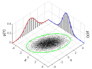
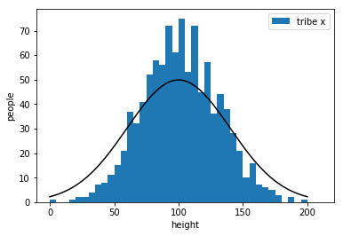
假設同一種東西分布為常態分布(Gaussian distribution)

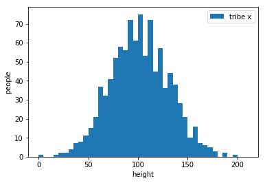
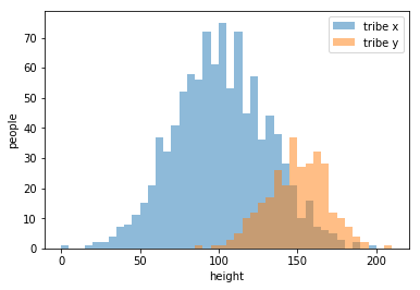
example:classify two tribes with their heights
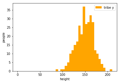
draw an appropriate curve to it

my strategy\(\cdots\)
楚河漢界
tribe x
tribe y
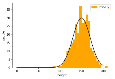
But how to get the curve?
determined by three features:
- \(\mu\):平均值、中心(公式)
- \(\Sigma\):分布的寬度(公式)
- height:高度(population of tribe)
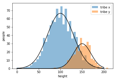
Gaussian Distribution:
\(f_{\mu,\Sigma}(x)=\frac{1}{(2\pi)^{\frac{D}{2}}}\frac{1}{|\Sigma|^\frac{1}{2}}exp\{-\frac{1}{2}(x-\mu)^T\Sigma^{-1}(x-\mu)\}\)
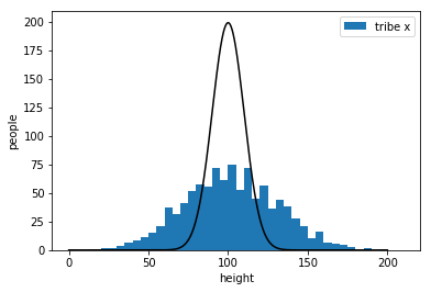
若中心為\(\mu\),寬度為\(\Sigma\),部落人口為\(n\):
distribution:\(f_{\mu,\Sigma}(x)\)(只考慮分布區域範圍)
curve:\(n\times f_{\mu,\Sigma}(x)\)(曲線方程式)
what exactly \(f(x)\) means ?
tribe x's \(f(x)\):
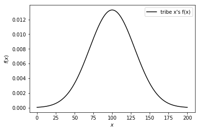
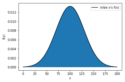
曲線下面積\(=1\)
\(f(a)\)代表多少比例的人分布在 \(x=a\)
find the best
\(\Rightarrow\) maximize "goodness"
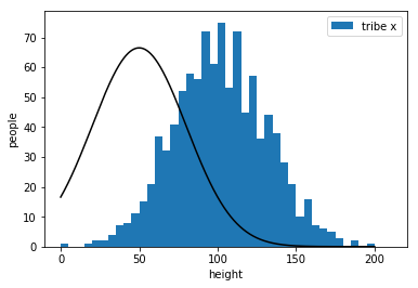
bad
bad

better

worst
almost there
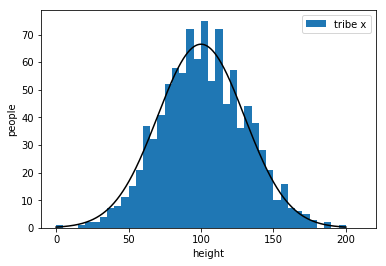
the best !!!
Gaussian Distribution:
\(f_{\mu,\Sigma}(x)=\frac{1}{(2\pi)^{\frac{D}{2}}}\frac{1}{|\Sigma|^\frac{1}{2}}exp\{-\frac{1}{2}(x-\mu)^T\Sigma^{-1}(x-\mu)\}\)
consider the i-th class \((C_i)\)
找到最好的\((\mu_i,\Sigma_i)\)來描述第 \(i\) 類的分布
define "the best":maximum \(G_i(\mu,\Sigma)\)
goodness \(=G_i(f_{\mu,\Sigma})=\prod_{k\in C_i} f_{\mu,\Sigma}(k)\)
\(\mu_i=\frac{1}{|C_i|}\sum\limits_{x\in C_i}x\)
\(\Sigma_i=\frac{1}{|C_i|}\sum\limits_{x\in C_i}(x-\mu_i)(x-\mu_i)^T\)
Gaussian Distribution:
\(f_{\mu,\Sigma}(x)=\frac{1}{(2\pi)^{\frac{D}{2}}}\frac{1}{|\Sigma|^\frac{1}{2}}exp\{-\frac{1}{2}(x-\mu)^T\Sigma^{-1}(x-\mu)\}\)
找到所有class的機率分布(curve)後:
\(P_i(x):=(x\) 屬於第 \(i\) 類的機率\()\)
\(P_i(x)=\frac{|C_i|\times f_{\mu_i,\Sigma_i}(x)}{\sum\limits_k(|C_k|\times f_{\mu_k,\Sigma_k}(x))}\)
機率分布對集合大小加權後再計算占比
?
\(135\sim 140\)
60%
12%
28%
\(130\sim 135\)
22%
33%
45%
Logistic Regression
\(\Longrightarrow\)假設輸出只有yes/no兩類
先做一個小小的假設\(\cdots\)令\(\Sigma_0=\Sigma_1=\Sigma\)
我也還不知道為什麼\(\cdots\)
\(P_0(x)=\frac{|C_0|\times f_{\mu_0,\Sigma_0}(x)}{|C_0|\times f_{\mu_0,\Sigma_0}+|C_1|\times f_{\mu_1,\Sigma_1}}\)
\(P_1(x)=1-P_0(x)\)
\(P_0(x)=\frac{|C_0|\times f_{\mu_0,\Sigma_0}(x)}{|C_0|\times f_{\mu_0,\Sigma_0}(x)+|C_1|\times f_{\mu_1,\Sigma_1}(x)}\)
\(=\frac{1}{1+\frac{|C_1|\times f_{\mu_1,\Sigma_1}(x)}{|C_0|\times f_{\mu_0,\Sigma_0}(x)}}\)
令\(\sigma(x)=\frac{1}{1+e^{-x}}\) , \(z=\ln{\frac{|C_0|\times f_{\mu_0,\Sigma_0}(x)}{|C_1|\times f_{\mu_1,\Sigma_1}(x)}}\)
\(P_0(x)=\frac{1}{1+\frac{|C_1|\times f_{\mu_1,\Sigma_1}(x)}{|C_0|\times f_{\mu_0,\Sigma_0}(x)}}=\sigma(z)\)
\(\ln{\frac{f_{\mu_0,\Sigma_0}(x)}{f_{\mu_1,\Sigma_1}(x)}}\)
\(=\ln{\frac{\frac{1}{(2\pi)^{\frac{D}{2}}}\frac{1}{|\Sigma|^\frac{1}{2}}exp\{-\frac{1}{2}(x-\mu_0)^T\Sigma^{-1}(x-\mu_0)\}}{\frac{1}{(2\pi)^{\frac{D}{2}}}\frac{1}{|\Sigma|^\frac{1}{2}}exp\{-\frac{1}{2}(x-\mu_1)^T\Sigma^{-1}(x-\mu_1)\}}}\)
\(=-\frac{1}{2}(x-\mu_0)^T\Sigma^{-1}(x-\mu_0)+\frac{1}{2}(x-\mu_1)^T\Sigma^{-1}(x-\mu_1)\)
\((x-\mu)^T\Sigma^{-1}(x-\mu)\)
\(=x^T\Sigma^{-1}x\underline{-x^T\Sigma^{-1}\mu-\mu^T\Sigma^{-1}x}+\mu^T\Sigma^{-1}\mu\)
\(=x^T\Sigma^{-1}x-2\mu^T\Sigma^{-1}x+\mu^T\Sigma^{-1}\mu\)
\(=-\frac{1}{2}(\underline{x^T\Sigma^{-1}x}-2\mu_0^T\Sigma^{-1}x+\mu_0^T\Sigma^{-1}\mu_0\\ -\underline{x^T\Sigma^{-1}x}+2\mu_1^T\Sigma^{-1}x-\mu_1^T\Sigma^{-1}\mu_1)\)
\(=-\frac{1}{2}(-2\mu_0^T\Sigma^{-1}x+\mu_0^T\Sigma^{-1}\mu_0+2\mu_1^T\Sigma^{-1}x-\mu_1^T\Sigma^{-1}\mu_1)\)
\(=(\mu_0-\mu_1)^T\Sigma^{-1}x+\frac{1}{2}(-\mu_0^T\Sigma^{-1}\mu_0+\mu_1^T\Sigma^{-1}\mu_1)\)
\(=\underline{(\mu_0-\mu_1)^T\Sigma^{-1}}x+\underline{\frac{1}{2}(-\mu_0^T\Sigma^{-1}\mu_0+\mu_1^T\Sigma^{-1}\mu_1)+\ln{\frac{|C_0|}{|C_1|}}}\)
\(z=\ln{\frac{|C_0|\times f_{\mu_0,\Sigma_0}(x)}{|C_1|\times f_{\mu_1,\Sigma_1}(x)}}\)
\(=\ln{\frac{|C_0|}{|C_1|}}+\ln{\frac{f_{\mu_0,\Sigma_0}(x)}{f_{\mu_1,\Sigma_1}(x)}}\)
\(=\underline{w}\cdot x+\underline{b}\)
\(P_0(x)=\sigma(z)=\sigma(w\cdot x+b)\)
\(x_1\)
\(x_2\)
\(x_n\)
\(\cdots\)
\(w_1\)
\(w_2\)
\(w_n\)
\(+b\)
\(\sigma\)
output
\(\sigma(x)=\frac{1}{1+e^{-x}}\)
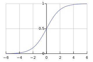
Sigmoid function
\(0\leq\sigma(x)\leq 1\)
訓練單一類神經元
1.設計函數集合
possibility \(=f_{w,b}(x)=\sigma(w\cdot x+b)\)
\(f_{w,b}(x)\geq 0.5\Rightarrow\) true
\(f_{w,b}(x)<0.5\Rightarrow\) false
找到最佳的 \(w,b\)
訓練單一類神經元
2.定義誤差函數
讓所有\(y_i\)是true 的\(f(x_i)\)接近\(1\)
讓所有\(y_i\)是false的\(f(x_i)\)接近\(0\)
均方誤差?
\(L(f)=\frac{1}{n}\sum(f(x_i)-y_i)^2\)
NO!!!
maximize 全對機率
\(y_i=0\Rightarrow p=1-f(x_i)\)
\(y_i=1\Rightarrow p=f(x_i)\)
將 \(p\) 連乘 \(=\prod p=\) 全對機率
maximize \(\prod p\Leftrightarrow\) minimize \(-\ln(\prod p)=-\sum(\ln p)\)
\(-\sum\ln p=-\sum(y_i)\ln f(x_i)+(1-y_i)\ln(1-f(x_i))\)
\((y_i)\ln f(x_i)+(1-y_i)\ln(1-f(x_i))\\=(0)\ln f(x_i)+(1-0)\ln(1-f(x_i))\\=\ln(1-f(x_i))\)
if \(y_i=0\)
\((y_i)\ln f(x_i)+(1-y_i)\ln(1-f(x_i))\\=(1)\ln f(x_i)+(1-1)\ln(1-f(x_i))\\=\ln f(x_i)\)
if \(y_i=1\)
\(-\sum\ln p=-\sum(y_i)\ln f(x_i)+(1-y_i)\ln(1-f(x_i))\)
令\(c(f(x_i),y_i)\\=-(y_i)\ln f(x_i)-(1-y_i)\ln(1-f(x_i))\)
cross entropy (\(H(p,q)\))
\(p,q\) 代表兩個機率分布描述
\(H(p,q)=-\sum\limits_{x\in X}p(x)\log q(x)\)
\(H(p,q)\) 代表 \(p,q\) 的差異
\(L(f_{w,b})=\frac{1}{n}\sum c(f_{w,b}(x_i),y_i)\)
分布 \(p\)
分布 \(q\)
\(p(X=0)=1-y\)
\(p(X=1)=y\)
\(q(X=0)=1-f(x)\)
\(q(X=1)=f(x)\)
cross entropy \(=H(y,f(x)),c(f(x),y)\)
\(X=\{0,1\}\)
\(L(f_{w,b})=\frac{1}{n}\sum c(f_{w,b}(x_i),y_i)\)
訓練單一類神經元
3.調整函數
\(w_i'=w_i-\eta \frac{\partial L(f)}{\partial w_i}\)
\(b'=b-\eta \frac{\partial L(f)}{\partial b}\)
\(\frac{\partial L(f_{w,b})}{\partial w_i}=\frac{\partial L(f_{w,b})}{\partial f_{w,b}(x)}\frac{\partial f_{w,b}(x)}{\partial w_i}=\frac{1}{n}\sum\frac{\partial c(f_{w,b}(x),y)}{\partial f_{w,b}(x)}\frac{\partial f_{w,b}(x)}{\partial w_i}\)
\(\frac{\partial c(f_{w,b}(x),y)}{\partial f_{w,b}(x)}=-\frac{\partial y\ln f_{w,b}(x)}{\partial f_{w,b}(x)}-\frac{\partial(1-y)\ln(1-f_{w,b}(x))}{\partial f_{w,b}(x)}\)
\(=-\frac{y}{f_{w,b}(x)}+\frac{1-y}{1-f_{w,b}(x)}=-\frac{y}{\sigma(z)}+\frac{1-y}{1-\sigma(z)}\)
\(\frac{\partial f_{w,b}(x)}{\partial w_i}=\frac{\partial\sigma(z)}{\partial w_i}=\frac{\partial\sigma(z)}{\partial z}\frac{\partial z}{\partial w_i}=\frac{\partial\sigma(z)}{\partial z}x_i\)
\(\frac{\partial\sigma(z)}{\partial z}=\frac{\partial(\frac{1}{1+e^{-z}})}{\partial(1+e^{-z})}\frac{\partial(1+e^{-z})}{\partial z}=\frac{\partial(\frac{1}{1+e^{-z}})}{\partial(1+e^{-z})}\frac{\partial e^{-z}}{\partial z}\)
\(=-\frac{1}{(1+e^{-z})^2}\cdot(-e^{-z})=\sigma(z)(1-\sigma(z))\)
\(\frac{\partial L(f_{w,b})}{\partial w_i}\)
\(=\frac{1}{n}\sum(-\frac{y}{\sigma(z)}+\frac{1-y}{1-\sigma(z)})(\sigma(z)(1-\sigma(z))x_i)\)
\(=\frac{1}{n}\sum -y(1-\sigma(z))x_i+(1-y)\sigma(x)x_i\)
\(=\frac{1}{n}\sum (\sigma(z)-y)x_i=\frac{1}{n}\sum(f_{w,b}(x)-y)x_i\)
wow 好漂亮的結果
\(\frac{\partial L(f_{w,b})}{\partial w_i}=\sum (f_{w,b}(x)-y)x_i\)
\(w_i'=w_i-\frac{\eta}{n}\sum (f_{w,b}(x)-y)x_i\)
\(b'=b-\frac{\eta}{n}\sum(f_{w,b}(x)-y)\)
linear v.s. logistic
linear regression
logistic regression
function set
loss function
differential
\(f_{w,b}(x)=w\cdot x+b\)
\(f_{w,b}(x)=\sigma(w\cdot x+b)\)
\(L(f_{w,b})=\frac{1}{n}\sum\limits_i(f_{w,b}(x_i)-y_i)^2\)
\(L(f_{w,b})=\frac{1}{n}\sum\limits_i c(f_{w,b}(x_i),y_i)\)
\(\frac{\partial L(f_{w,b})}{\partial w_j}=\frac{2}{n}\sum\limits_i(f_{w,b}(x_i)-y_i)(x_j)\)
\(\frac{\partial L(f_{w,b})}{\partial w_j}=\frac{1}{n}\sum\limits_i(f_{w,b}(x_i)-y_i)(x_j)\)
Let's train!!!
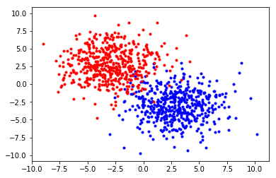
訓練資料
import matplotlib.colors as colors
import matplotlib.cm as cm
from matplotlib import animation, rc
from IPython.display import HTML
from mpl_toolkits.mplot3d import Axes3D
import matplotlib.pyplot as plt
import numpy as np
import pandas as pd
import time
url = 'https://thomasinfor.github.io/train-data/logistic_regression1.csv'
data = pd.read_csv(url)
n=len(data['x'])
temp=[data['x'],data['y']]
train_x=np.array([[temp[0][i],temp[1][i]] for i in range(n)])
train_y=np.array(data['class'])
plt.scatter([train_x[i][0] for i in range(n) if train_y[i]==0],
           [train_x[i][1] for i in range(n) if train_y[i]==0],c="red",s=3)
plt.scatter([train_x[i][0] for i in range(n) if train_y[i]==1],
           [train_x[i][1] for i in range(n) if train_y[i]==1],c="blue",s=3)
plt.show()
訓練資料
定義各種函數
# define functions
def sigmoid(x):
    return 1/(1+np.exp(-x))
# inner product
def dot(w,x):
    total=0
    for i in range(2):
        total=total+w[i]*x[i]
    return total
# function set
def f(w,b,x):
    return sigmoid(dot(w,x)+b)
# cross entropy (single loss)
def cross_entropy(a,b):
    if b==0 or b==1:
        return abs(a-b)*1000000000
    return -np.exp(b)*a-np.exp(1-b)*(1-a)
# loss function (summation over all data loss)
def loss(w,b):
    total=0;
    for i in range(n):
        total+=cross_entropy(f(w,b,train_x[i]),train_y[i])
    return total/n
# defferential
def dldw(w,b,i):
    total=0
    for j in range(n):
        total=total+(f(w,b,train_x[j])-train_y[j])*train_x[j][i]
    return total/n
# defferentail
def dldb(w,b):
    total=0
    for j in range(n):
        total=total+(f(w,b,train_x[j])-train_y[j])
    return total/n
# predict answer (return predicted class)
def predict(w,b,x):
    if f(w,b,x)>=0.5:
        return 1
    else:
        return 0
# predict all data
def test_all(w,b,x,y):
    cnt=0
    for i in range(len(x)):
        if predict(w,b,x[i])==y[i]:
            cnt+=1
    return cnt/len(x)
開始訓練!
# training !!!
w,b=[0.1,0.1],1
history={'w':[w],'b':[b],'loss':[loss(w,b)],'acc':[test_all(w,b,train_x,train_y)]}
learning_rate=0.01
iters=1000
print("start training")
start=time.time()
for cnt in range(iters):
last=list(w)
for i in range(2):
w[i]-=learning_rate*dldw(last,b,i)
b-=learning_rate*dldb(last,b)
history['w'].append(list(w))
history['b'].append(b)
history['loss'].append(loss(w,b))
history['acc'].append(test_all(w,b,train_x,train_y))
print("finished")
end=time.time()
print(f"time: {end-start} seconds")
print(f"result: w = {w}, b = {b}")
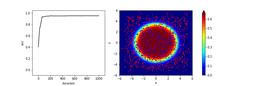
print(f"accuracy: {test_all(w,b,train_x,train_y)*100}%")訓練結果
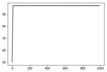
accuracy:97.09%
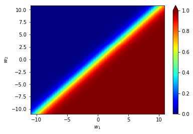
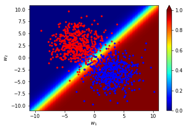
訓練結果
# plotting result
# you can just ignore this part when
# you're reading as an beginner
fig, ax = plt.subplots(1,2)
fig.patch.set_alpha(0)
fig.set_size_inches(fig.get_figwidth()*2,fig.get_figheight())
plt.close()
ax[0].set_xlim(-iters*0.1,iters*1.1)
ax[0].set_ylim(-0.1*max(history['acc']),max(history['acc'])*1.1)
X = np.linspace(-15,15,100)
X, Y = np.meshgrid(X, X)
Z = Y * 0
Z=f(history['w'][0],history['b'][0],[X,Y])
pcm = ax[1].pcolor(X, Y, Z, norm=colors.Normalize(vmin=Z.min(), vmax=Z.max()), cmap=cm.jet)
fig.colorbar(pcm, ax=ax, extend='max')
ax[0].set_xlabel('$iteration$')
ax[0].set_ylabel('$acc$')
ax[1].set_xlabel('$x$')
ax[1].set_ylabel('$y$')
x0, y0 = [], []
line0, = ax[0].plot([],[],c='black')
def animate(i):
Z=f(history['w'][int(i)],history['b'][int(i)],[X,Y])
ax[1].pcolor(X, Y, Z, norm=colors.Normalize(vmin=Z.min(), vmax=Z.max()), cmap=cm.jet)
ax[1].scatter([train_x[i][0] for i in range(n) if train_y[i]==0],
[train_x[i][1] for i in range(n) if train_y[i]==0],c="red",s=3)
ax[1].scatter([train_x[i][0] for i in range(n) if train_y[i]==1],
[train_x[i][1] for i in range(n) if train_y[i]==1],c="blue",s=3)
x0.append(i)
y0.append(history['acc'][int(i)])
line0.set_data(x0,y0)
return (line0,)
anim = animation.FuncAnimation(fig, animate, frames=200, interval=30, blit=True)
rc('animation', html='jshtml')
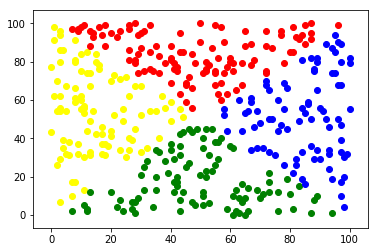
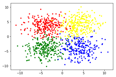
animmulti-class classification
\(x_1\)
\(x_2\)
\(x_n\)
\(\cdots\)
\(+b_1\)
\(\cdots\)
\(+b_2\)
\(+b_3\)
\(+b_k\)
\(\sum=z_1\)
\(\sum=z_2\)
\(\sum=z_3\)
\(\sum=z_k\)
\(exp\)
\(exp\)
\(exp\)
\(exp\)
\(e^{z_1}\)
\(e^{z_2}\)
\(e^{z_3}\)
\(e^{z_k}\)
\(p_1=\frac{e^{z_1}}{\sum\limits_je^{z_j}}\)
\(p_2=\frac{e^{z_2}}{\sum\limits_je^{z_j}}\)
\(p_3=\frac{e^{z_3}}{\sum\limits_je^{z_j}}\)
\(p_k=\frac{e^{z_k}}{\sum\limits_je^{z_j}}\)
softmax
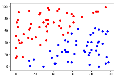
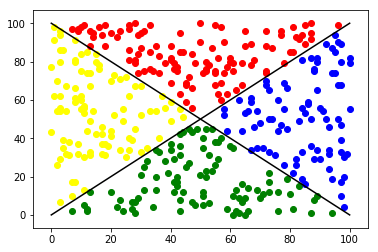
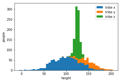
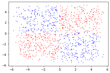
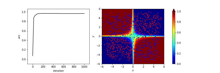
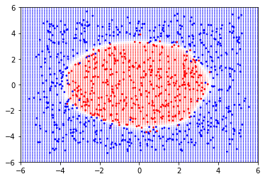
但是如果\(\cdots\)這種資料呢?
data
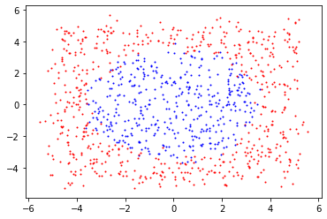
結果
accuracy:45.77%
結果
連我都看得出來的東西
他怎麼學不出來???
Disadvantage of Logistic Regression
- 前提假設高斯分布!!!
- 只有直的分界線
How to conquer it ?
- 特徵轉換(feature transformation)
- 類神經網路(neural network)!!!
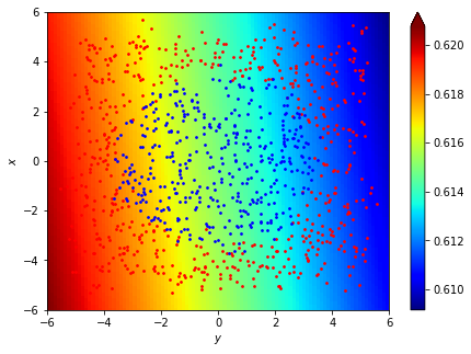
特徵轉換
\(x=(a,b)\rightarrow y\)
轉換\(\cdots\)
\(x'=(\sqrt{a^2+b^2})\rightarrow y\)
import matplotlib.colors as colors
import matplotlib.cm as cm
from matplotlib import animation, rc
from IPython.display import HTML
from mpl_toolkits.mplot3d import Axes3D
import matplotlib.pyplot as plt
import numpy as np
import pandas as pd
import time
url = 'https://thomasinfor.github.io/train-data/feature_extraction1.csv'
data = pd.read_csv(url)
n=len(data['x'])
temp=[data['x'],data['y']]
x_train=np.array([[temp[0][i],temp[1][i]] for i in range(n)])
y_train=np.array(data['class'])
plt.scatter([x_train[i][0] for i in range(n) if y_train[i]==0],
[x_train[i][1] for i in range(n) if y_train[i]==0],c="red",s=3)
plt.scatter([x_train[i][0] for i in range(n) if y_train[i]==1],
[x_train[i][1] for i in range(n) if y_train[i]==1],c="blue",s=3)
plt.show()
# define functions
# define functions
def sigmoid(x):
return 1/(1+np.exp(-x))
# inner product
def dot(w,x):
total=0
for i in range(1):
total=total+w[i]*x[i]
return total
# function set
def f(w,b,x):
return sigmoid(dot(w,x)+b)
# cross entropy (single loss)
def cross_entropy(a,b):
if b==0 or b==1:
return abs(a-b)*1000000000
return -np.exp(b)*a-np.exp(1-b)*(1-a)
# loss function (summation over all data loss)
def loss(w,b):
total=0;
for i in range(n):
total+=cross_entropy(f(w,b,feature[i]),y_train[i])
return total/n
# defferential
def dldw(w,b,i):
total=0
for j in range(n):
total=total+(f(w,b,feature[j])-y_train[j])*feature[j][i]
return total/n
# defferentail
def dldb(w,b):
total=0
for j in range(n):
total=total+(f(w,b,feature[j])-y_train[j])
return total/n
# predict answer (return predicted class)
def predict(w,b,x):
if f(w,b,x)>=0.5:
return 1
else:
return 0
# predict all data
def test_all(w,b,x,y):
cnt=0
for i in range(len(x)):
if predict(w,b,x[i])==y[i]:
cnt+=1
return cnt/len(x)
# feature extraction
def extract(x):
x=np.array(x)
if x.shape==(2,):
return np.array([np.sqrt(x[0]**2+x[1]**2)])
else:
xp=[]
for i in range(len(x)):
xp.append([np.sqrt(x[i][0]**2+x[i][1]**2)])
return np.array(xp)
x_train=np.array(x_train)
feature=extract(x_train)
# training !!!
w,b=[0.1],1
history={'w':[w],'b':[b],'loss':[loss(w,b)],'acc':[test_all(w,b,feature,y_train)]}
learning_rate=1
iters=1000
print("start training")
start=time.time()
for cnt in range(iters):
last=list(w)
for i in range(1):
w[i]-=learning_rate*dldw(last,b,i)
b-=learning_rate*dldb(last,b)
history['w'].append(list(w))
history['b'].append(b)
history['loss'].append(loss(w,b))
history['acc'].append(test_all(w,b,feature,y_train))
print("finished")
end=time.time()
print(f"time: {end-start} seconds")
print(f"result: w = {w}, b = {b}")
print(f"accuracy: {test_all(w,b,feature,y_train)*100}%")
# plot boundary
X = np.linspace(-6,6,100)
X, Y = np.meshgrid(X, X)
Z = X * 0
for i in range(len(X)):
for j in range(len(X)):
Z[i][j]=f(w,b,extract([X[i][j],Y[i][j]]))
fig, ax = plt.subplots(figsize=(7,5))
pcm = ax.pcolor(X, Y, Z, norm=colors.Normalize(vmin=Z.min(), vmax=Z.max()), cmap=cm.jet)
ax.scatter([x_train[i][0] for i in range(n) if y_train[i]==0],
[x_train[i][1] for i in range(n) if y_train[i]==0],c="red",s=3)
ax.scatter([x_train[i][0] for i in range(n) if y_train[i]==1],
[x_train[i][1] for i in range(n) if y_train[i]==1],c="blue",s=3)
fig.colorbar(pcm, ax=ax, extend='max')
ax.set_xlabel('$y$')
ax.set_ylabel('$x$')
plt.show()
# plotting result
# you can just ignore this part when
# you're reading as an beginner
fig, ax = plt.subplots(1,2)
fig.patch.set_alpha(0)
fig.set_size_inches(fig.get_figwidth()*2,fig.get_figheight())
plt.close()
ax[0].set_xlim(-iters*0.1,iters*1.1)
ax[0].set_ylim(-0.1*max(history['acc']),max(history['acc'])*1.1)
X = np.linspace(-6,6,100)
X, Y = np.meshgrid(X, X)
Z = Y * 0
for x in range(len(X)):
for y in range(len(X)):
Z[x][y]=f(history['w'][0],history['b'][0],extract([X[x][y],Y[x][y]]))
pcm = ax[1].pcolor(X, Y, Z, norm=colors.Normalize(vmin=Z.min(), vmax=Z.max()), cmap=cm.jet)
fig.colorbar(pcm, ax=ax, extend='max')
ax[0].set_xlabel('$iteration$')
ax[0].set_ylabel('$acc$')
ax[1].set_xlabel('$x$')
ax[1].set_ylabel('$y$')
x0, y0 = [], []
line0, = ax[0].plot([],[],c='black')
def animate(i):
for x in range(len(X)):
for y in range(len(X)):
Z[x][y]=f(history['w'][int(i)],history['b'][int(i)],extract([X[x][y],Y[x][y]]))
ax[1].pcolor(X, Y, Z, norm=colors.Normalize(vmin=Z.min(), vmax=Z.max()), cmap=cm.jet)
ax[1].scatter([x_train[i][0] for i in range(n) if y_train[i]==0],
[x_train[i][1] for i in range(n) if y_train[i]==0],c="red",s=3)
ax[1].scatter([x_train[i][0] for i in range(n) if y_train[i]==1],
[x_train[i][1] for i in range(n) if y_train[i]==1],c="blue",s=3)
x0.append(i)
y0.append(history['acc'][int(i)])
line0.set_data(x0,y0)
return (line0,)
anim = animation.FuncAnimation(fig, animate, frames=np.linspace(0,iters-1,50), interval=30, blit=True)
rc('animation', html='jshtml')
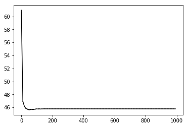
anim訓練結果
accuracy:95.6%
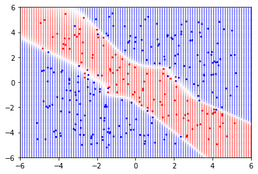
data
結果
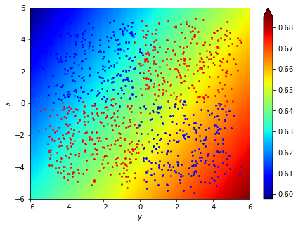
特徵轉換
\(x=(a,b)\rightarrow y\)
轉換\(\cdots\)
\(x'=(a\cdot b)\rightarrow y\)
import matplotlib.colors as colors
import matplotlib.cm as cm
from matplotlib import animation, rc
from IPython.display import HTML
from mpl_toolkits.mplot3d import Axes3D
import matplotlib.pyplot as plt
import numpy as np
import pandas as pd
import time
url = 'https://thomasinfor.github.io/train-data/feature_extraction2.csv'
data = pd.read_csv(url)
n=len(data['x'])
temp=[data['x'],data['y']]
x_train=np.array([[temp[0][i],temp[1][i]] for i in range(n)])
y_train=np.array(data['class'])
plt.scatter([x_train[i][0] for i in range(n) if y_train[i]==0],
           [x_train[i][1] for i in range(n) if y_train[i]==0],c="red",s=3)
plt.scatter([x_train[i][0] for i in range(n) if y_train[i]==1],
           [x_train[i][1] for i in range(n) if y_train[i]==1],c="blue",s=3)
plt.show()

# define functions
# define functions
def sigmoid(x):
    return 1/(1+np.exp(-x))
# inner product
def dot(w,x):
    total=0
    for i in range(1):
        total=total+w[i]*x[i]
    return total
# function set
def f(w,b,x):
    return sigmoid(dot(w,x)+b)
# cross entropy (single loss)
def cross_entropy(a,b):
    if b==0 or b==1:
        return abs(a-b)*1000000000
    return -np.exp(b)*a-np.exp(1-b)*(1-a)
# loss function (summation over all data loss)
def loss(w,b):
    total=0;
    for i in range(n):
        total+=cross_entropy(f(w,b,feature[i]),y_train[i])
    return total/n
# defferential
def dldw(w,b,i):
    total=0
    for j in range(n):
        total=total+(f(w,b,feature[j])-y_train[j])*feature[j][i]
    return total/n
# defferentail
def dldb(w,b):
    total=0
    for j in range(n):
        total=total+(f(w,b,feature[j])-y_train[j])
    return total/n
# predict answer (return predicted class)
def predict(w,b,x):
    if f(w,b,x)>=0.5:
        return 1
    else:
        return 0
# predict all data
def test_all(w,b,x,y):
    cnt=0
    for i in range(len(x)):
        if predict(w,b,x[i])==y[i]:
            cnt+=1
    return cnt/len(x)
# feature extraction
def extract(x):
    x=np.array(x)
    if x.shape==(2,):
        return np.array([x[0]*x[1]])
    else:
        xp=[]
        for i in range(len(x)):
            xp.append([x[i][0]*x[i][1]])
        return np.array(xp)
x_train=np.array(x_train)
feature=extract(x_train)

# training !!!
w,b=[10],10
history={'w':[w],'b':[b],'loss':[loss(w,b)],'acc':[test_all(w,b,feature,y_train)]}
learning_rate=1
iters=1000
print("start training")
start=time.time()
for cnt in range(iters):
    last=list(w)
    for i in range(1):
        w[i]-=learning_rate*dldw(last,b,i)
    b-=learning_rate*dldb(last,b)
    history['w'].append(list(w))
    history['b'].append(b)
    history['loss'].append(loss(w,b))
    history['acc'].append(test_all(w,b,feature,y_train))
print("finished")
end=time.time()
print(f"time: {end-start} seconds")
print(f"result: w = {w}, b = {b}")
print(f"accuracy: {test_all(w,b,feature,y_train)*100}%")

# plotting result
# you can just ignore this part when
# you're reading as an beginner
fig, ax = plt.subplots(1,2)
fig.patch.set_alpha(0)
fig.set_size_inches(fig.get_figwidth()*2,fig.get_figheight())
plt.close()
ax[0].set_xlim(-iters*0.1,iters*1.1)
ax[0].set_ylim(-0.1*max(history['acc']),max(history['acc'])*1.1)
X = np.linspace(-6,6,100)
X, Y = np.meshgrid(X, X)
Z = Y * 0
for x in range(len(X)):
    for y in range(len(X)):
        Z[x][y]=f(history['w'][0],history['b'][0],extract([X[x][y],Y[x][y]]))
pcm = ax[1].pcolor(X, Y, Z, norm=colors.Normalize(vmin=Z.min(), vmax=Z.max()), cmap=cm.jet)
fig.colorbar(pcm, ax=ax, extend='max')
ax[0].set_xlabel('$iteration$')
ax[0].set_ylabel('$acc$')
ax[1].set_xlabel('$x$')
ax[1].set_ylabel('$y$')
x0, y0 = [], []
line0, = ax[0].plot([],[],c='black')
def animate(i):
    for x in range(len(X)):
        for y in range(len(X)):
            Z[x][y]=f(history['w'][int(i)],history['b'][int(i)],extract([X[x][y],Y[x][y]]))
    ax[1].pcolor(X, Y, Z, norm=colors.Normalize(vmin=Z.min(), vmax=Z.max()), cmap=cm.jet)
    ax[1].scatter([x_train[i][0] for i in range(n) if y_train[i]==0],
        [x_train[i][1] for i in range(n) if y_train[i]==0],c="red",s=3)
    ax[1].scatter([x_train[i][0] for i in range(n) if y_train[i]==1],
        [x_train[i][1] for i in range(n) if y_train[i]==1],c="blue",s=3)
    x0.append(i)
    y0.append(history['acc'][int(i)])
    line0.set_data(x0,y0)
    return (line0,)
anim = animation.FuncAnimation(fig, animate, frames=np.linspace(0,iters-1,50), interval=30, blit=True)
rc('animation', html='jshtml')
anim
訓練結果
accuracy:96.4%
特徵轉換?
- 我怎麼知道怎麼轉換?
- 我會轉換我就自己分類就好了啊!
- 不能自己學怎麼轉換嗎?
| 人工轉換 | 機器學習 | |
| 時機 | 已知一些規律,較熟悉 | 無法找到規律 |
| 方法 | 預處理轉換 | 類神經網路!! |
Deep Learning
終於來了
| 人工轉換 | 機器學習 | |
| 時機 | 已知一些規律,較熟悉 | 無法找到規律 |
| 方法 | 預處理轉換 | 類神經網路!! |
\(x_1\)
\(x_2\)
\(x_3\)
\(x_4\)
\(x_5\)
\(\Sigma_1\)
\(\sigma(\Sigma_1+b_1)=P_1\)
\(w_1\)
\(w_2\)
\(w_3\)
\(w_4\)
\(w_5\)
\(h_1\)
\(h_2\)
recognizing feature 1
recognizing feature 2
\(h_3\)
\(h_4\)
recognizing feature 3 according to feature 1 and 2
recognizing feature 4 according to feature 1 and 2
\(y_1\)
\(y_2\)
make decisions according to feature 3 and 4
example - judging gender
黑色面積多?
身高高?
音頻高?
黑色線條多?
移動速度?

強壯?
長髮?
It's actually a black box.
We don't know what machine recognizes as features.

INPUT
HIDDEN
OUTPUT
\(x_0\)
\(x_1\)
\(x_2\)
\(x_3\)
\(x_4\)
\(a_0\)
\(a_1\)
\(a_2\)
\(a_3\)
\(a_4\)
\(a_5\)
\(a_6\)
\(b_0\)
\(b_1\)
\(b_2\)
\(b_3\)
\(b_4\)
\(b_5\)
\(b_6\)
\(c_0\)
\(c_1\)
\(c_2\)
\(c_3\)
\(c_4\)
\(c_5\)
\(c_6\)
\(y_0\)
\(y_1\)
\(y_2\)
matrix evaluation
\(a_1\)
\(a_2\)
\(a_3\)
\(a_4\)
\(b_1\)
\(b_2\)
\(a_i\)
\(w_{ij}\)
\(b_j\)
b_1=a_1w_{11}+a_2w_{12}+a_3w_{13}+a_4w_{14}
b_2=a_1w_{21}+a_2w_{22}+a_3w_{23}+a_4w_{24}
\begin{bmatrix}
b_1\\
b_2\\
b_3
\end{bmatrix}_{3\times 1}
=
\begin{bmatrix}
w_{11} & w_{21} & w_{31} & w_{41}\\
w_{12} & w_{22} & w_{32} & w_{42}\\
w_{13} & w_{23} & w_{33} & w_{43}
\end{bmatrix}_{3\times 4}
\begin{bmatrix}
a_1\\
a_2\\
a_3\\
a_4
\end{bmatrix}_{4\times 1}
b_3=a_1w_{31}+a_2w_{32}+a_3w_{33}+a_4w_{34}
\(b_3\)
\begin{bmatrix}
b_1\\
b_2\\
b_3
\end{bmatrix}_{3\times 1}
=
\begin{bmatrix}
w_{11} & w_{21} & w_{31} & w_{41}\\
w_{12} & w_{22} & w_{32} & w_{42}\\
w_{13} & w_{23} & w_{33} & w_{43}
\end{bmatrix}_{3\times 4}
\begin{bmatrix}
a_1\\
a_2\\
a_3\\
a_4
\end{bmatrix}_{4\times 1}
\begin{bmatrix}
b_1 & b_2 & b_3
\end{bmatrix}_{1\times 3}
=
\begin{bmatrix}
a_1 & a_2 & a_3 & a_4
\end{bmatrix}_{1\times 4}
\begin{bmatrix}
w_{11} & w_{12} & w_{13}\\
w_{21} & w_{22} & w_{23}\\
w_{31} & w_{32} & w_{33}\\
w_{41} & w_{42} & w_{43}
\end{bmatrix}_{4\times 3}
\(W^T\)
\(A^T\)
\(B^T\)
\(B\)
\(A\)
\(W\)
電腦可以快速地計算矩陣(張量tensor)
\(x_0\)
\(x_1\)
\(x_2\)
\(x_3\)
\(x_4\)
\(a_0\)
\(a_1\)
\(a_2\)
\(a_3\)
\(a_4\)
\(a_5\)
\(a_6\)
\(b_0\)
\(b_1\)
\(b_2\)
\(b_3\)
\(b_4\)
\(b_5\)
\(b_6\)
\(c_0\)
\(c_1\)
\(c_2\)
\(c_3\)
\(c_4\)
\(c_5\)
\(c_6\)
\(y_0\)
\(y_1\)
\(y_2\)
\(X\)
\(W_1\)
\(W_2\)
\(W_3\)
\(W_4\)
\(Y\)
\(X\)
\(W_1\)
\(\sigma(\)
\()\)
\(W_2\)
\(\sigma(\)
\()\)
\()\)
\()\)
\(\sigma(\)
\(W_3\)
\(W_4\)
\(\sigma(\)
\(=\)
\(Y\)
\(x_0\)
\(x_1\)
\(x_2\)
\(x_3\)
\(x_4\)
\(a_0\)
\(a_1\)
\(a_2\)
\(a_3\)
\(a_4\)
\(a_5\)
\(a_6\)
\(c_0\)
\(c_1\)
\(c_2\)
\(c_3\)
\(c_4\)
\(c_5\)
\(c_6\)
\(y_0\)
\(y_1\)
\(y_2\)
\(\cdots\)
so
many
layers
Backpropagation
反向傳播
1.function set
\(x_0\)
\(x_1\)
\(x_2\)
\(x_3\)
\(x_4\)
\(a_0\)
\(a_1\)
\(a_2\)
\(a_3\)
\(a_4\)
\(a_5\)
\(a_6\)
\(b_0\)
\(b_1\)
\(b_2\)
\(b_3\)
\(b_4\)
\(b_5\)
\(b_6\)
\(c_0\)
\(c_1\)
\(c_2\)
\(c_3\)
\(c_4\)
\(c_5\)
\(c_6\)
\(y_0\)
\(y_1\)
\(y_2\)
2.loss function
INPUT
OUTPUT

\text{probability distribution}=\left[\text{cat},\text{dog},\text{bird}\right]
\left[1,0,0\right]

\left[0,0,1\right]

\left[0,1,0\right]
2.loss function
\(y_0\)
\(y_1\)
\(y_2\)
\(0.01\)
\(0.23\)
\(0.76\)
\(0\)
\(0\)
\(1\)
ans
cross entropy
output
In information theory, the cross entropy between two probability distributions \(p\) and \(q\) over the same underlying set of events measures the average number of bits needed to identify an event drawn from the set if a coding scheme used for the set is optimized for an estimated probability distribution \(q\), rather than the true distribution \(p\).
在資訊理論中,基於相同事件測度的兩個概率分布 \(p\) 和 \(q\) 的交叉熵是指,當基於一個「非自然」(相對於「真實」分布 \(p\) 而言)的概率分布 \(q\) 進行編碼時,在事件集合中唯一標識一個事件所需要的平均比特數(bit)。
2.loss function
\texttt{OUTPUT: }\left[y_1,y_2,\cdots,y_k\right]\\
\texttt{ANSWER: }\left[\hat{y_1},\hat{y_2},\cdots,\hat{y_k}\right]
\texttt{loss=}-\frac{1}{n}\sum\limits_{i=0}^{n}(\sum\limits_{j=0}^{k}\hat{y_j^i}\log y_j^i)
3.update parameters\(\cdots\)
\(x_0\)
\(x_1\)
\(x_2\)
\(x_3\)
\(x_4\)
\(a_0\)
\(a_1\)
\(a_2\)
\(a_3\)
\(a_4\)
\(a_5\)
\(a_6\)
\(b_0\)
\(b_1\)
\(b_2\)
\(b_3\)
\(b_4\)
\(b_5\)
\(b_6\)
\(c_0\)
\(c_1\)
\(c_2\)
\(c_3\)
\(c_4\)
\(c_5\)
\(c_6\)
\(y_0\)
\(y_1\)
\(y_2\)
這要怎麼微分???
calculate gradient
\(a_1\)
\(v_1\)
\frac{\partial C}{\partial v_1}=\frac{\partial b_1}{\partial v_1}\frac{\partial C}{\partial b_1}=a_1\frac{\partial C}{\partial b_1}

\(\sum\)
\(b_1\)
\(\sum\)
\(b_2\)
\(a_2\)
\(c_1\)
\(w_1\)
\(\sum\)
\(d_1\)
\(\sum\)
\(d_2\)
\(c_2\)
\(\cdots\) \(C\)
\frac{\partial C}{\partial b_1}=\frac{\partial c_1}{\partial b_1}(\frac{\partial d_1}{\partial c_1}\frac{\partial C}{\partial d_1}+\frac{\partial d_2}{\partial c_1}\frac{\partial C}{\partial d_2})=\\
\frac{\partial \sigma(b_1)}{\partial b_1}(w_1\frac{\partial C}{\partial d_1}+w_2\frac{\partial C}{\partial d_2})=\sigma'(b_1)(w_1\frac{\partial C}{\partial d_1}+w_2\frac{\partial C}{\partial d_2})\\
=\sigma(b_1)(1-\sigma(b_1))(w_1\frac{\partial C}{\partial d_1}+w_2\frac{\partial C}{\partial d_2})
\(w_2\)
calculate gradient
\(a_1\)
\(v_1\)
\frac{\partial C}{\partial v_1}=a_1\sigma'(b_1)(w_1\frac{\partial C}{\partial d_1}+w_2\frac{\partial C}{\partial d_2})
\(\sum\)
\(b_1\)
\(\sum\)
\(b_2\)
\(a_2\)
\(c_1\)
\(w_1\)
\(\sum\)
\(d_1\)
\(\sum\)
\(d_2\)
\(c_2\)
\(\cdots\) \(C\)
\(w_2\)
\(w_1\)
\(w_2\)
\frac{\partial C}{\partial d_1}
\frac{\partial C}{\partial d_2}
\frac{\partial C}{\partial b_1}=\sigma'(b_1)(w_1\frac{\partial C}{\partial d_1}+w_2\frac{\partial C}{\partial d_2})
w_1\frac{\partial C}{\partial d_1}+w_2\frac{\partial C}{\partial d_2}
\frac{\partial C}{\partial b_2}=\sigma'(b_2)(w_3\frac{\partial C}{\partial d_1}+w_4\frac{\partial C}{\partial d_2})
w_3\frac{\partial C}{\partial d_1}+w_4\frac{\partial C}{\partial d_2}
\(w_3\)
\(w_4\)
calculate gradient
\hat{y_1}
\hat{y_2}
\frac{\partial C}{\partial y_2}
\frac{\partial C}{\partial y_1}
C
\frac{\partial C}{\partial d_2}
\frac{\partial C}{\partial d_1}
\frac{\partial C}{\partial c_2}
\frac{\partial C}{\partial c_1}
\frac{\partial C}{\partial b_2}
\frac{\partial C}{\partial b_1}
\frac{\partial C}{\partial a_2}
\frac{\partial C}{\partial a_1}
\(\cdots\)
將梯度往反方向傳播--反向傳播 back propagation
反向傳播 back propagation = 鏈鎖律 chain rule
來點實作吧!
等等 我要寫出那些東西?!
Keras
講課好難
1.定義函數集合
model = Sequential()model.add(Dense(25,input_shape=(2,),activation='sigmoid'))先宣告
\(\cdots\)
25個
model.add(Dense(25,activation='sigmoid'))\(\cdots\)
25個
\(\cdots\)
25個
model.add(Dense(1,activation='sigmoid'))\(\cdots\)
25個
\(\cdots\)
25個
model.summary()Model: "sequential_128"
_________________________________________________________________
Layer (type) Output Shape Param #
=================================================================
dense_392 (Dense) (None, 25) 75
_________________________________________________________________
dense_393 (Dense) (None, 25) 650
_________________________________________________________________
dense_394 (Dense) (None, 1) 26
=================================================================
Total params: 751
Trainable params: 751
Non-trainable params: 0
_________________________________________________________________2.定義誤差函數
3-1.計算梯度
model.compile(loss='binary_crossentropy',optimizer=SGD())誤差函數
使用
隨機梯度下降法
Stochastic
Gradient
Descent
'binary_crossentropy'
# ylogY+(1-y)log(1-Y)
'categorical_entropy'
# 很多東西的交叉熵
'mse'
# 均方誤差
...
SGD(...)
Adam(...)
RMSprop(...)
Adagrad(...)3-2.更新函數
model.fit(x,y,batch_size,epochs,verbose=1)
# x: 訓練資料的x
# y: 訓練資料的y
# batch_size: 就是batch_size
# epochs: 要跑過整個訓練資料幾次(iterations)
# 更多參數可以參考keras的documentation
# verbose: 要不要印出訓練過程
Epoch 1/10
1000/1000 [==============================] - 1s 910us/step - loss: 0.7360
Epoch 2/10
1000/1000 [==============================] - 0s 19us/step - loss: 0.6937
Epoch 3/10
1000/1000 [==============================] - 0s 19us/step - loss: 0.6938
Epoch 4/10
1000/1000 [==============================] - 0s 26us/step - loss: 0.6930
Epoch 5/10
1000/1000 [==============================] - 0s 16us/step - loss: 0.6925
Epoch 6/10
1000/1000 [==============================] - 0s 21us/step - loss: 0.6927
Epoch 7/10
1000/1000 [==============================] - 0s 22us/step - loss: 0.6929
Epoch 8/10
1000/1000 [==============================] - 0s 17us/step - loss: 0.6927
Epoch 9/10
1000/1000 [==============================] - 0s 20us/step - loss: 0.6935
Epoch 10/10
1000/1000 [==============================] - 0s 22us/step - loss: 0.6930看結果
print(model.evaluate(x,y,verbose=1))1000/1000 [==============================] - 0s 414us/step
0.6922322082519531print(model.predict([[1,2],[3,4],[5,6],[7,8]]))
# print(model.predict(x))[[9.9988043e-01]
[4.0138029e-03]
[8.0009222e-06]
[1.1767075e-06]]
# array of model's prediction來試試這張圖吧
import matplotlib.pyplot as plt
from matplotlib import cm
import numpy as np
import pandas as pd

url = 'https://thomasinfor.github.io/train-data/feature_extraction1.csv'
data = pd.read_csv(url)
n=len(data['x'])
x_train=np.array([[data['x'][i],data['y'][i]] for i in range(n)])
y_train=np.array(data['class'])
plt.scatter([x_train[i][0] for i in range(n)],
            [x_train[i][1] for i in range(n)],
            c=y_train,cmap=cm.bwr,s=3,vmin=0,vmax=1)
plt.show()
import keras
from keras.layers import Dense
from keras.optimizers import SGD
from keras.models import Sequential
from keras.callbacks import LambdaCallback
# not important
def result(model,xlim,ylim,prtdata=True,density=100):
coord=[[x,y] for x in np.linspace(-xlim,xlim,density) for y in np.linspace(-ylim,ylim,density)]
coord=np.array(coord)
res=model.predict(coord)
res=[i[0] for i in res]
plt.xlim(-xlim,xlim)
plt.ylim(-ylim,ylim)
plt.scatter([coord[i][0] for i in range(len(coord))],[coord[i][1] for i in range(len(coord))],c=res,cmap=cm.bwr,s=0.3,vmin=0,vmax=1)
if prtdata:
plt.scatter([x_train[i][0] for i in range(n)],
[x_train[i][1] for i in range(n)],
c=y_train,cmap=cm.bwr,s=3,vmin=0,vmax=1)
plt.show()
# 1.function set
model=Sequential()
model.add(Dense(25,input_shape=(2,),activation='sigmoid'))
model.add(Dense(25,activation='sigmoid'))
model.add(Dense(1,activation='sigmoid'))
# 2.define loss 3-1.calculate gradient
model.compile(loss='binary_crossentropy',optimizer=SGD(0.9),metrics=['accuracy'])
# print function
model.summary()
# not important
def func(epoch,logs):
if epoch%50==0:
print(epoch,':',sep='')
result(model,6,6,False)
plot=LambdaCallback(on_epoch_end=func)
# 3-2.update function
model.fit(x_train,y_train,batch_size=100,epochs=500,callbacks=[plot],verbose=0)
# print result
print(model.evaluate(x_train,y_train))
result(model,6,6)很簡單吧!
試試這兩個吧!
url = 'https://thomasinfor.github.io/train-data/feature_extraction2.csv'url = 'https://thomasinfor.github.io/train-data/feature_extraction3.csv'import keras
from keras.layers import Dense
from keras.optimizers import SGD
from keras.models import Sequential
from keras.callbacks import LambdaCallback
# not important
def result(model,xlim,ylim,prtdata=True,density=100):
coord=[[x,y] for x in np.linspace(-xlim,xlim,density) for y in np.linspace(-ylim,ylim,density)]
coord=np.array(coord)
res=model.predict(coord)
res=[i[0] for i in res]
plt.xlim(-xlim,xlim)
plt.ylim(-ylim,ylim)
plt.scatter([coord[i][0] for i in range(len(coord))],[coord[i][1] for i in range(len(coord))],c=res,cmap=cm.bwr,s=0.3,vmin=0,vmax=1)
if prtdata:
plt.scatter([x_train[i][0] for i in range(n)],
[x_train[i][1] for i in range(n)],
c=y_train,cmap=cm.bwr,s=3,vmin=0,vmax=1)
plt.show()
# 1.function set
model=Sequential()
model.add(Dense(...,input_shape=(2,),activation='sigmoid'))
model.add(Dense(...,activation='sigmoid'))
...
model.add(Dense(1,activation='sigmoid'))
# 2.define loss 3-1.calculate gradient
model.compile(loss='binary_crossentropy',optimizer=SGD(...),metrics=['accuracy'])
# print function
model.summary()
# not important
def func(epoch,logs):
if epoch%50==0:
print(epoch,':',sep='')
result(model,6,6,False)
plot=LambdaCallback(on_epoch_end=func)
# 3-2.update function
model.fit(x_train,y_train,batch_size=50,epochs=...,callbacks=[plot],verbose=0)
# print result
print(model.evaluate(x_train,y_train))
result(model,6,6)小技巧們
model=Sequential()
model.add(Dense(25,input_shape=(2,),activation='relu'))
model.add(Dense(25,activation='relu'))
model.add(Dense(1,activation='sigmoid'))
ReLU
- 收斂快速:不需要很多epochs才能train好
- 深度加深,一樣有效:適合深度學習
gradient vanishing
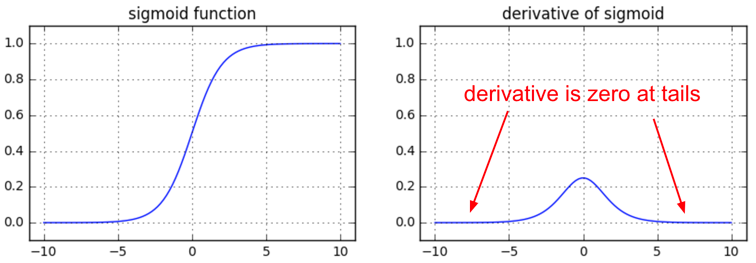
sigmoid function => 梯度容易變很小 => 不易更新函數
ReLU
f(x)=
\begin{cases}
x & x>0\\
0 & x\leq0
\end{cases}\\
=max(0,x)
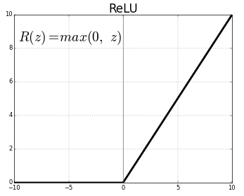
線性:不會有梯度消失的問題
powerful optimizers
RMSprop(...)
Adagrad(...)
Adam(...)
很強很好用!
validation data
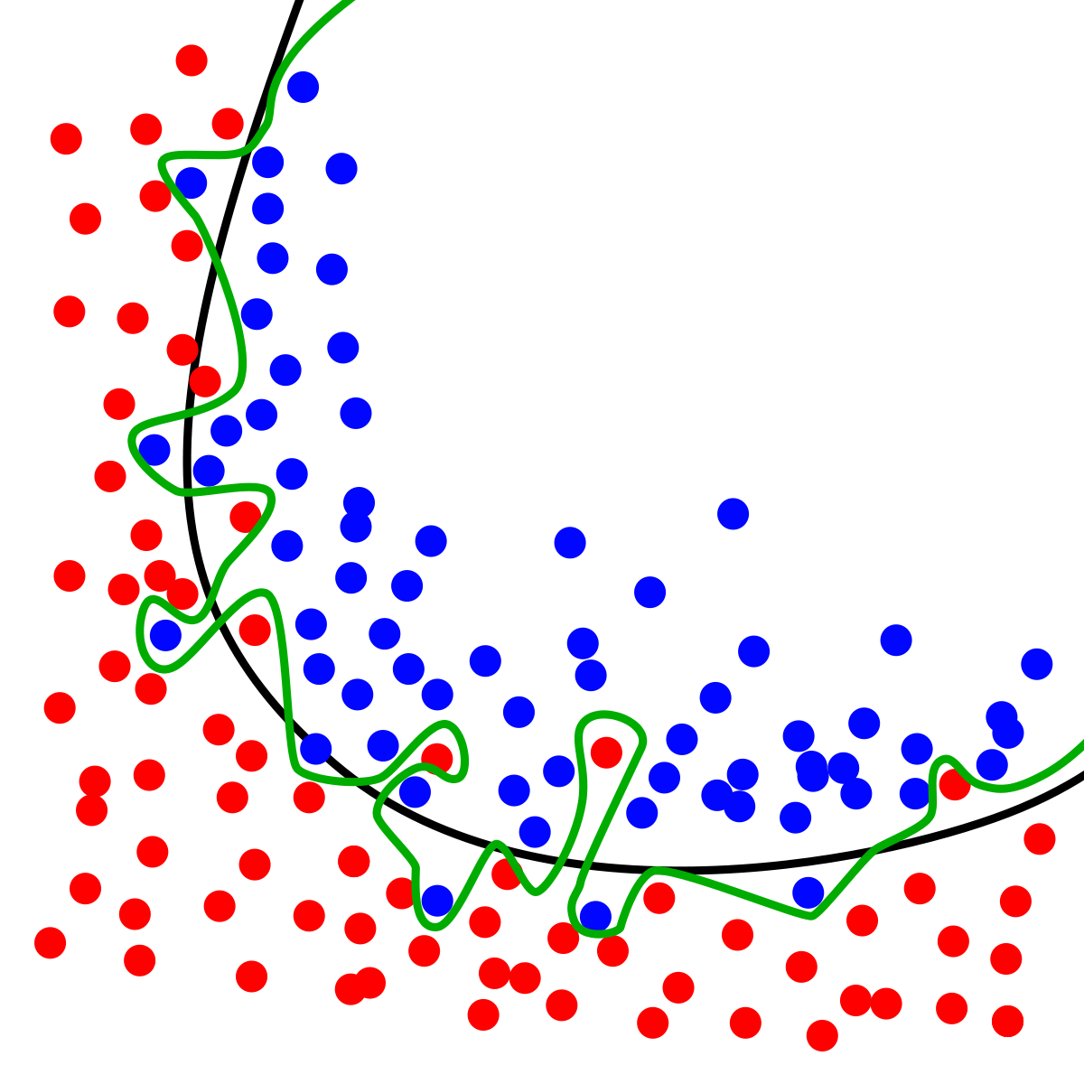
model.fit(x,y,validation_split=0.2)解決過適(overfitting)問題
overfitting?
what we expect
early stopping
用training data以外的東西來檢查它有沒有過適
----你沒有辦法「過適」你沒看過的東西!
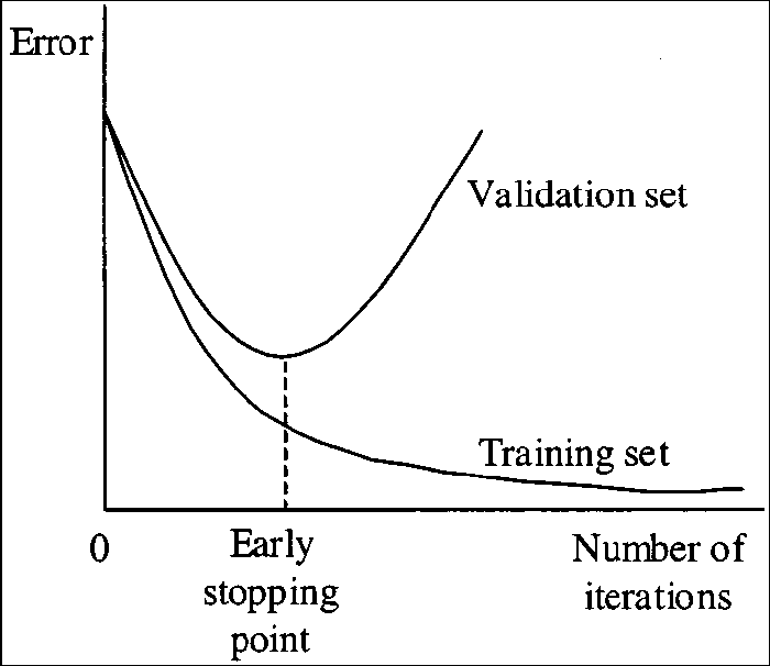
在overfitting前
就停止訓練
每天都是不同的你
Dropout
抓爆
\(x_0\)
\(x_1\)
\(a_0\)
\(a_1\)
\(a_2\)
\(a_3\)
\(b_0\)
\(b_1\)
\(b_2\)
\(b_3\)
\(c_0\)
\(c_1\)
\(c_2\)
\(c_3\)
\(y_0\)
\(y_1\)
- randomly disable some neurons by \(p\%\) (hyperparameter)
- different structure everytime \(\Rightarrow\) hard to overfit
- train neurons more independently
- train multiple network,combine them as result (ensemble)
數量\(\times\)權重\(=(1-p\% )\times w=(1)\times w'\)
model.add(Dense(128))
model.add(Dropout(0.5))
model.add(Dense(128))
regularization
常規化
- 參數接近零 \(\Rightarrow\) 函數較平滑 \(\Rightarrow\) 常規化
\(L'(f_\theta)=L(f_\theta)+||\theta||_1=L(f_\theta)+\sum|\theta_i|\)
L1 norm
\(L'(f_\theta)=L(f_\theta)+||\theta||_2=L(f_\theta)+\sum(\theta_i)^2\)
L2 norm
Keras 其他功能介紹
列表
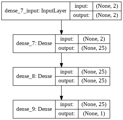
plot_model
- 畫出模型的簡圖!
from keras.utils import plot_model
plot_model(model)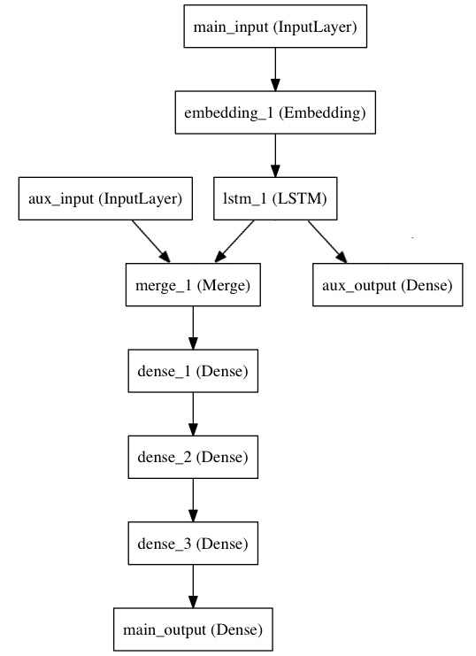
model.save(path)
model = load_model(path)
- 儲存、載入訓練好的模型吧!
from keras.models import load_model
model.save('my_model.h5')
del model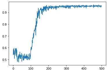
model=load_model('my_model.h5')- 取得訓練時accuray和loss的變化
history=model.fit(x,y)
print(history)
# then we can...
plt.plot(history.history['acc'])
plt.show()
history=model.fit()
keras.applications
爽啦!偷別人東西
functional API
Sequential \(\Leftrightarrow\) functional
堆疊型 \(\Leftrightarrow\) 函數型
# sequential
model=Sequential()
model.add(Dense(128,input_shape=(10,)))
model.add(Dropout(0.5))
model.add(Dense(128))
# functional
input_layer=Input(sgape=(10,))
hidden1=Dense(128)(input_layer)
hidden2=Dropout(0.5)(hidden1)
output_layer=Dense(128)(hidden2)
model=Model(input_layer,output_layer)functional API
把layer當做一個函數!
layer1
layer2
fully
connected
\(\Rightarrow\)
layer1
layer2
\(f\)
\(f(\text{layer1})=\text{layer2}\\\text{Dense}(\text{layer1})=\text{layer2}\)
layer2=Dense(...)(layer2)functional API
# 第一個輸入
input1=Input(shape=(10,))
x1=Dense(128)(input1)
x1=Dense(128)(x1)
x1=Dense(32)(x1)
# 第二個輸入
input2=Input(shape=(8,))
x2=Dense(32)(input2)
x2=Dense(32)(x2)
x2=Dense(32)(x2)
# 將處理過的兩個輸入接起來
con=concatenate([x1,x2])
con=Dense(28)(con)
# 接出第一個輸出
x=Dense(64)(con)
output1=Dense(1)(x)
# 接出第二個輸出
x=Dense(16)(con)
output2=Dense(1)(x)
# 建構(2輸入)->(2輸出)的模型
model=Model([input1,input2],
            [output1,output2])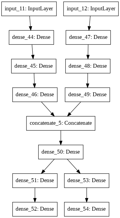
MNIST
實作好玩嗎
MNIST 手寫數字資料庫
MNIST in ML = "hello world" in C++

from keras.datasets import mnistimport keras
from keras.layers import Dense
from keras.optimizers import SGD
from keras.models import Sequential
from keras.datasets import mnist
# input image dimensions
img_rows, img_cols = 28, 28
num_classes=10
# the data, split between train and test sets
(x_train, y_train), (x_test, y_test) = mnist.load_data()
x_train = x_train.reshape(x_train.shape[0], img_rows * img_cols)
x_test = x_test.reshape(x_test.shape[0], img_rows * img_cols)
x_train = x_train.astype('float32')
x_test = x_test.astype('float32')
x_train /= 255
x_test /= 255
print('x_train shape:', x_train.shape)
print(x_train.shape[0], 'train samples')
print(x_test.shape[0], 'test samples')
# convert class vectors to binary class matrices
y_train = keras.utils.to_categorical(y_train, num_classes)
y_test = keras.utils.to_categorical(y_test, num_classes)
model=Sequential()
model.add(Dense(10,input_shape=(784,),activation='softmax'))
model.compile(loss='categorical_crossentropy',optimizer=SGD(),metrics=['accuracy'])
model.summary()
model.fit(x_train,y_train,epochs=10,batch_size=32)preprocessing datas
自己試試看吧
model = Sequential()宣告模型
model.add(Dense(128,
                activation='relu',
                input_shape=(img_rows*img_cols,)))
add a hidden layer with 128 neurons
\(\cdots 128\cdots\)
model.add(Dense(128,
                activation='relu')
add a hidden layer with 128 neurons
model.add(Dense(128,
                activation='relu')
add a hidden layer with 128 neurons
\(\cdots 128\cdots\)
\(\cdots 128\cdots\)
INPUT
(input_shape)
model.add(Dense(num_classes,
                activation='softmax'))
add an output layer with 10 neurons (10 categories)
\(\cdots 10\cdots\)
model.compile(loss=keras.losses.categorical_crossentropy,
              optimizer=SGD(),
              metrics=['accuracy'])
define loss function , optimize with stochastic gradient descent
model.fit(x_train, y_train,
          batch_size=batch_size,
          epochs=epochs,
          verbose=1)
train with x_train and y_train
epochs = repeat times
score = model.evaluate(x_test, y_test, verbose=0)
print('Test loss:', score[0])
print('Test accuracy:', score[1])
evaluate accuracy and loss with x_test and y_test
model.summary()print model
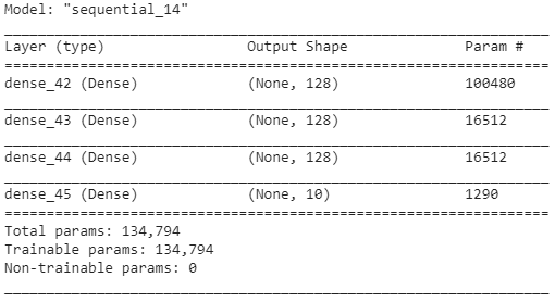
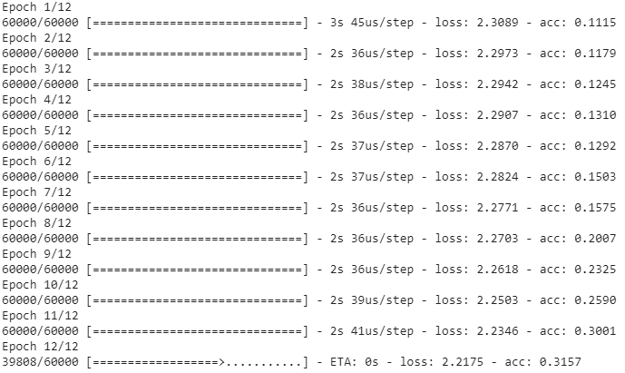
result
import matplotlib.pyplot as plt
plt.plot(history.history['acc'])
plt.xlabel('epochs')
plt.ylabel('accuracy')
plt.show()
plt.plot(history.history['loss'])
plt.xlabel('epochs')
plt.ylabel('loss')
plt.show()
train acc: 0.9956 test acc: 0.9775
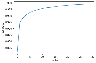
幫我試出(想出)
這幾個東西有什麼影響!
- batch_size
- 深度
- 每層神經元數
predict
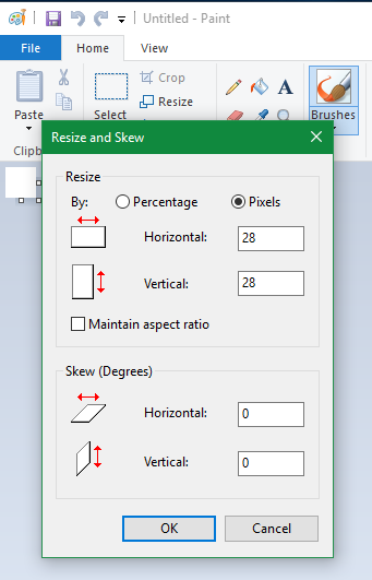
小畫家--在\(28\times 28\)的方格內畫數字

upload it
predict
import matplotlib.pyplot as plt
import numpy as np

def rgb2gray(rgb):
    return np.dot(rgb[...,:3], [0.299, 0.587, 0.114])

FILE = 'replace this with your uploaded file name'
source = rgb2gray(plt.imread(FILE))
source = 1-source

result = model.predict(source.reshape(1,img_cols*img_rows))

print('Result:', result.argmax())
plt.imshow(source)
plt.show()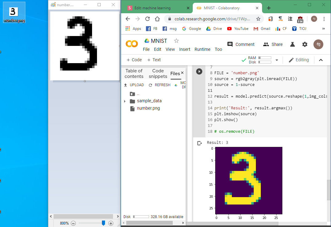
CNN
convolutional neural network
捲積
神經網路
內積
inner product
\(*\)
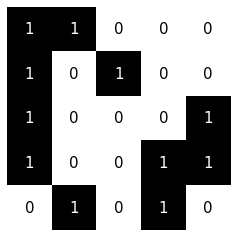
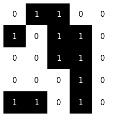
\(=\)
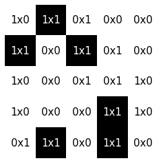
內積:兩個形狀一樣的東西對應相乘再加起來
\(=6\)
內積
inner product
每個神經元都在做捲積
\rbrace
權重不同的內積
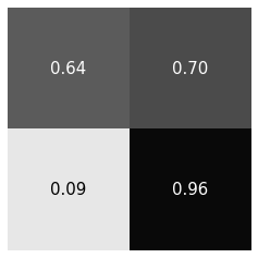
內積
內積可以找出特定的pattern

\(*\)
\(=5\)
\(=4.50\)
\(=-10.19\)
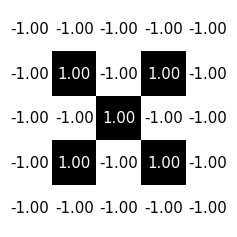
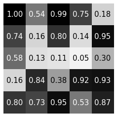
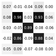
filter
BUT...
\(*\)
\(=5\)
\(=-1\)
\(=-5\)
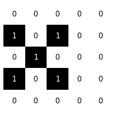
SO...
這樣我們不就需要這九個filter...?
Text
浪費!
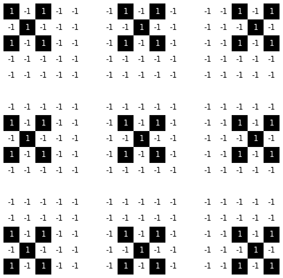
有更輕鬆的方法
同一個小filter用很多次!
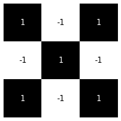

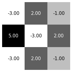
大東西和小東西做很多次內積\(\Rightarrow\)捲積
很簡單對吧XD
聽不懂的話我道歉
其實這很像神經網路
這九個神經元:
- 共用權重
- 僅連接九格(
fully connected) - 參數量少、訓練容易
總而言之
CNN的使用時機:
- 相同的pattern可能出現在很多地方
CNN的優點:
- 減少參數量
- 適合用於圖片辨識
用法!
model.add(Conv2D(units,kernal_size,padding=''))
# units: filter的數量
# kernal_size: pattern的大小
# padding: 'valid'=一般 , 'same'=保持大小
用法!
model=Sequential()
model.add(Conv2D(128,(3,3),padding='same',
                 input_shape=(28,28,1)))
model.add(Activation('relu'))
model.add(Conv2D(128,(3,3),padding='same'))
model.add(Activation('relu'))
model.add(Flatten())
model.add(Dense(10))
model.add(Activation('softmax'))
model.compile(loss='sparse_categorical_crossentropy',
              optimizer=Adam(),metrics=['accuracy'])
model.summary()
load data
import keras
from keras.layers import Dense,Conv2D,Activation,Flatten
from keras.models import Sequential
from keras.optimizers import Adam
from keras.datasets import mnist
(x_train,y_train),(x_test,y_test)=mnist.load_data()
print(x_train.shape)
print(y_train.shape)
print(x_test.shape)
print(y_test.shape)
x_train=x_train.reshape(x_train.shape+(1,))/255
x_test=x_test.reshape(x_test.shape+(1,))/255
fashion_mnist
多練習!
from keras.datasets import fashion_mnist
(x_train, y_train), (x_test, y_test) = fashion_mnist.load_data()
x_train = x_train.reshape(x_train.shape + (1,))
x_test = x_test.reshape(x_test.shape + (1,))
大家加油!
分享一下
最後一堂課!
影片自動配音效AI
machine learning
By thomaswang2003
machine learning
星期三放學社課


